This is an update to Agent Economics: a BOTEC on feasibility. Toby Ord pointed me to Gus Hamilton's Weibull reanalysis of the METR data. Hamilton finds that a declining hazard rate (Weibull with κ ≈ 0.6–0.9 for SOTA models) may fit the data as well as Ord's constant hazard rate, producing a much fatter survival tail that changes the economics. This post presents both models and extends the analysis in two directions: a quantitative treatment of verification cost as the binding constraint under the Weibull model, and a systematic examination of the economic conditions under which a genuinely dangerous autonomous agent could actually operate. His full comment is in Appendix A.

Calculators for this post

I built two interactive calculators to accompany this post. 

• The Half-Life Tax calculator lets you toggle between the exponential and Weibull survival functions, adjust all parameters, and explore sensitivity analysis.
• The Economic Anatomy calculator focuses on verification economics, self-sustaining agent viability, reckless deployment costs, and the full four-condition chain.

BLUF:

• Agent costs grow superlinearly with task length while human costs grow linearly, creating a reliability wall that cheaper inference cannot overcome.
• The only thing that moves this wall is how long an agent can stay on track, and the only thing that changes its shape is how reliability decays over time.
• Scaling makes agents faster and more accurate per step, but does not appear to change the structure of how they accumulate errors on long tasks, which is likely an architectural property. This is because current agents do fresh inference over a growing context window at each step.
• Human verification, not compute, is the dominant cost for complex tasks.
• These dynamics mean month-long autonomous plans do not reach coin-flip reliability until roughly January 2029 on current trends.
• An AI bubble correction would extend these timelines further.
• The economics naturally favour bounded, verified, short-horizon deployments and buy meaningful time for safety work, but this safety margin collapses if someone cracks continual learning and agents start maintaining coherence over long tasks the way humans do.

Summary: 

The original post modelled agent cost per successful outcome scaling exponentially with task length under Ord's constant hazard rate, while human cost scales linearly. This update incorporates Hamilton's Weibull alternative, under which agent costs scale as a stretched exponential rather than a pure exponential. The cost wall is gentler, but it is still a wall. The dominant parameter remains the agent's reliability horizon (T₅₀). The available data does not yet show the shape of the reliability decay (κ) improving with model scale, though the sample is small and the estimates uncertain.

The other point I want to make is to trace the implications for a question that safety discussions often treat as purely technical: what are the economic conditions under which a dangerous autonomous agent actually gets to run? An agent that poses existential-level risks needs compute to operate. Compute costs money. Someone has to pay. That economic relationship creates constraints that are, I think, underappreciated in the safety literature.

The conclusion of this post is a timeline analysis. I argue that κ is an architectural property, not a scaling property, and that it will remain near 0.70 without a qualitative change in how models work. If that is correct, I can calculate when each category of dangerous autonomous agent becomes economically viable given the METR doubling trend. The answer: bounded multi-week agent tasks for companies reach viability by late 2027 to mid 2028. Self-sustaining agent-verifier pairs can plausibly bootstrap from late 2027, though with high failure rates on their own setup plans. Month-long autonomous plans do not reach even 25% reliability until early 2028, and do not reach 50% until January 2029. Three-month plans remain below 10% success until mid 2028. These timelines would compress by 7–16 months if κ improves to 0.50, and the dangerous regime would already be here if κ were at human levels (0.37). This is why κ is the variable to watch.

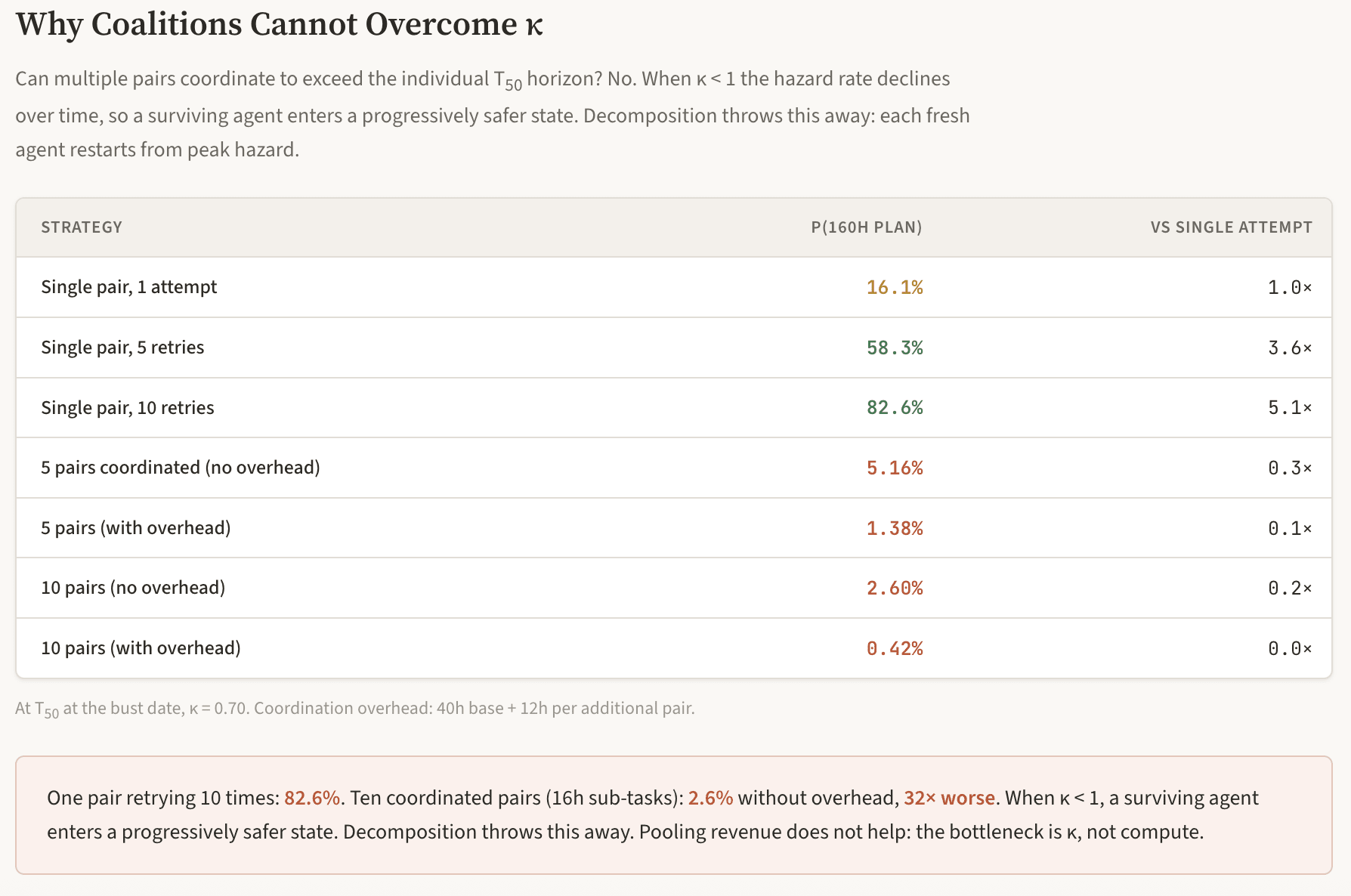
A bubble correction that slows the T₅₀ doubling trend would extend these timelines substantially. I estimate roughly 40 to 50% probability of a meaningful correction (capex growth falling below 15% or contracting absolutely) by end of 2027, and 55 to 70% by end of 2028, though a full telecom-style collapse is less likely (15 to 25%) than a deceleration. Even a deceleration from 7-month to 14-month doubling delays the most dangerous milestones by one to two years. A deeper stall to 24-month doubling (the telecom-precedent scenario) delays them by two or more years. Strikingly, inference cost changes barely matter for the dangerous milestones, because verification (human labour) dominates total cost at realistic review fractions. And self-sustaining pairs that have already bootstrapped survive even extreme price increases. But a correction also delays the κ breakthrough itself, by cutting the speculative architectural research that a continual learning paradigm would require. Coalitions of pairs cannot overcome the κ ceiling: decomposing a long plan across multiple agents is strictly worse than a single agent retrying, because the declining hazard rate (κ < 1) means each fresh agent restarts from the high initial failure rate (see Appendix B).

Important: this post does not address misuse of AI agents!

The setup

Toby Ord's "Half-Life" analysis (2025) showed that AI agent success rates on tasks decay with task length in a pattern analogous to radioactive decay. Using METR's 2025 data on software engineering and reasoning tasks, he proposed that a constant hazard rate model fits the observed decline: if an agent completes a 1-hour task with 50% probability, it completes a 2-hour task with roughly 25% and a 4-hour task with about 6%. Ord was careful to note that this was "suggestive" rather than proven, and has since updated that Hamilton is "probably right" that the hazard rate declines.

Hamilton's reanalysis fits a Weibull survival function, which introduces a shape parameter κ. When κ = 1 you recover the exponential; when κ < 1 the hazard rate decreases over time, meaning agents that survive the early part of a task become progressively less likely to fail per unit time. Hamilton finds κ ≈ 0.6–0.9 for SOTA models and κ ≈ 0.37 for humans. The two models fit about equally well on available data but diverge dramatically at the tails, where we have very few measurements.

Hamilton frames this through the lens of Peto's Paradox: blue whales have vastly more cells than humans but do not get cancer at a proportionally higher rate, because they have evolved superior error-correction mechanisms. The question for AI agents is whether anything analogous can emerge from scaling alone.

The METR data showed the 50% time horizon (T₅₀) for the best agents was roughly 2.5–5 hours and had been doubling every roughly 7 months. The International AI Safety Report 2026 uses the same data and projects multi-day task completion by 2030 if the trend continues.

The model

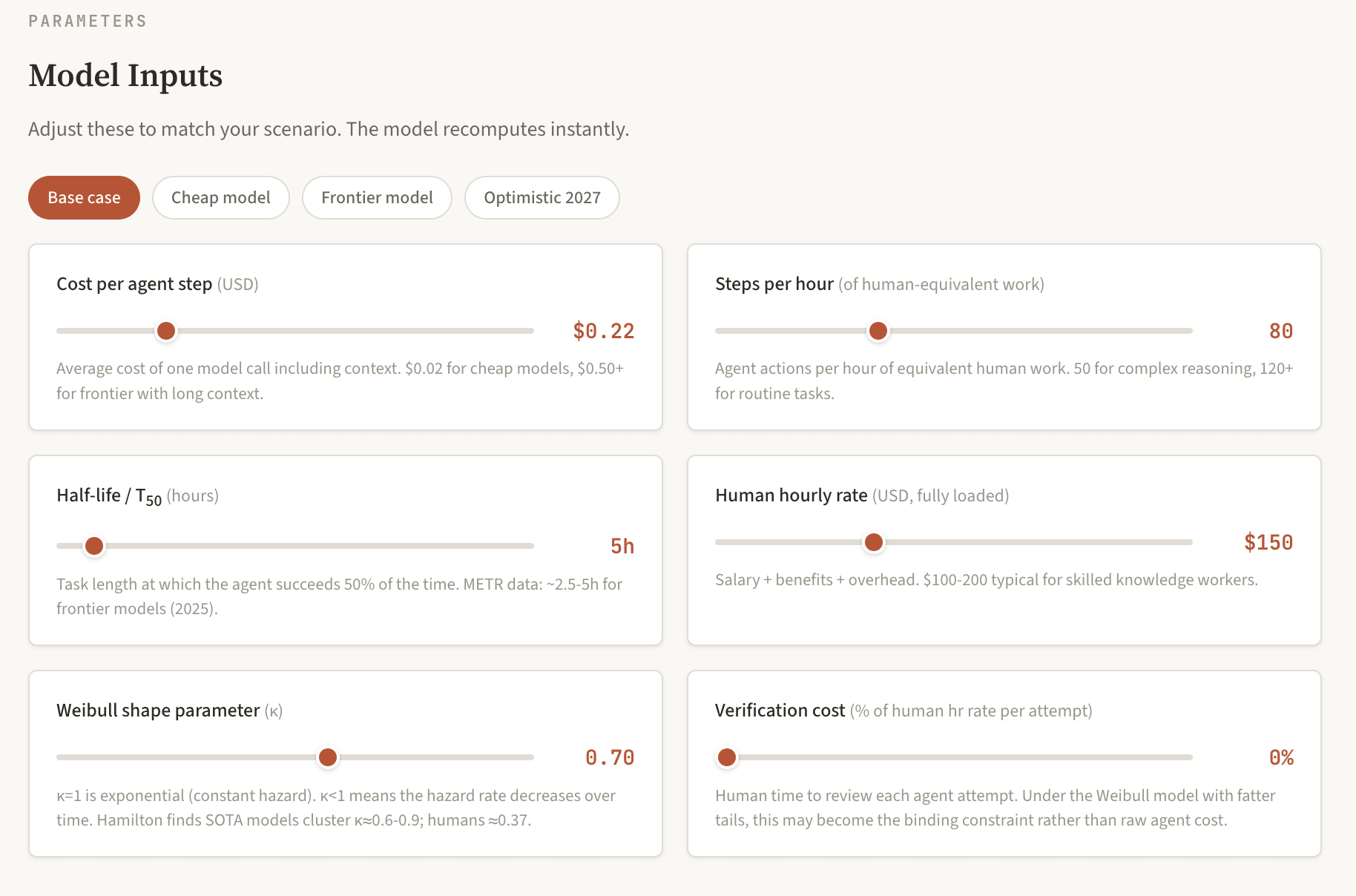
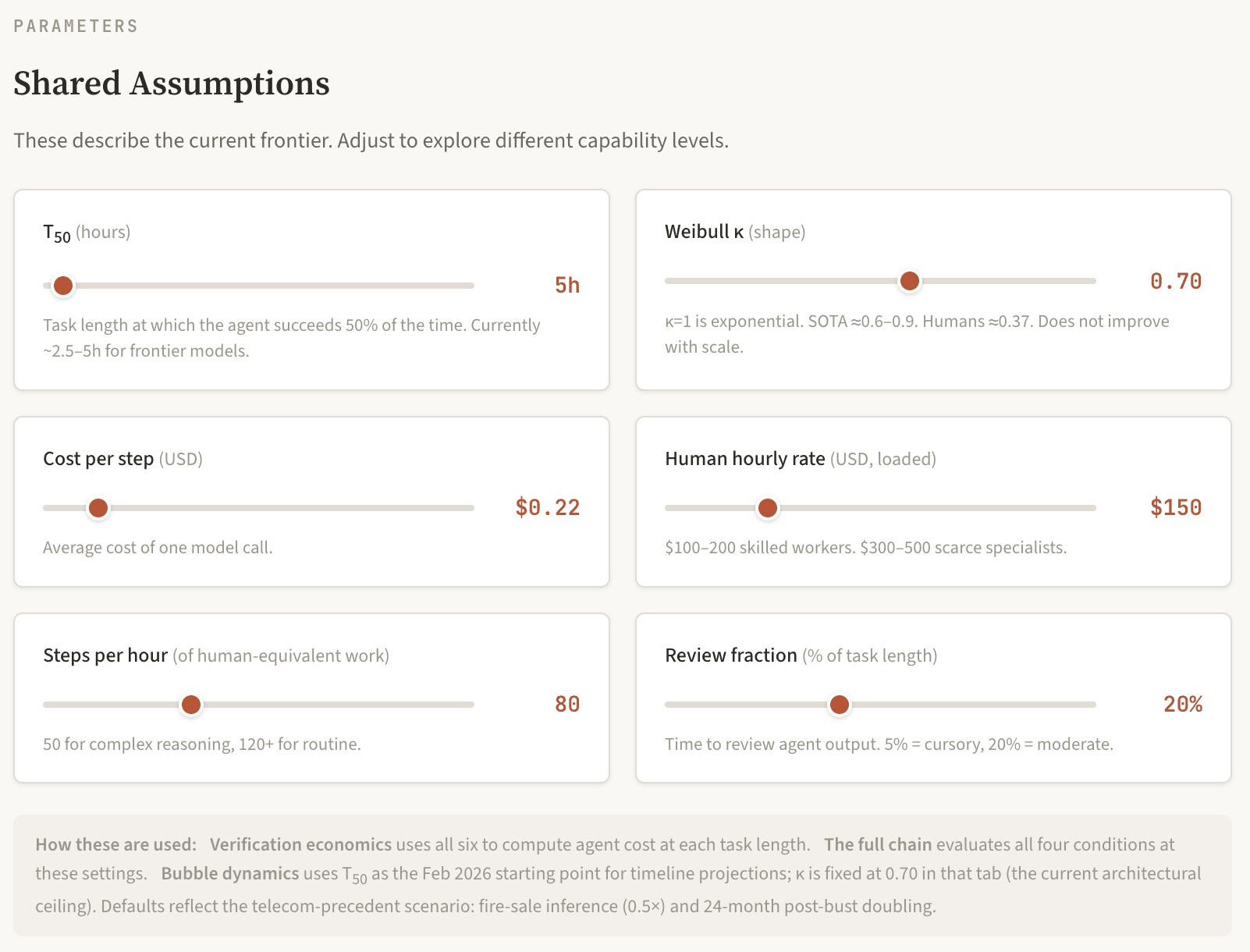
Six parameters drive the analysis.

• Cost per agent step ($): average cost of one model call including context. Ranges from roughly $0.02 (cheap model, short context) to roughly $0.55 (frontier, long context).
• Steps per hour of human-equivalent work: how many agent actions correspond to one hour of human task time. 50–120 depending on task complexity.
• T₅₀ (hours): task length at which the agent succeeds 50% of the time. Currently roughly 2.5–5h for frontier models on software tasks.
• Human hourly rate ($): fully loaded (salary + benefits + overhead). $100–200 for skilled knowledge workers.
• Weibull shape parameter (κ): 1.0 for exponential (constant hazard), 0.6–0.9 for SOTA models per Hamilton, 0.37 for humans.
• Verification cost: human time to review each agent attempt, modelled as a fraction of task length.

You can explore all of these parameters interactively. My Half-Life Tax calculator lets you toggle between the exponential and Weibull survival functions, adjust all six parameters, and see how the cost comparison and sensitivity analysis respond in real time.

The key equations:

Exponential model (Ord, κ = 1):

P(success) = 0.5^(task_hours / T₅₀)
E[attempts] = 2^(task_hours / T₅₀)

Weibull model (Hamilton, κ < 1):

λ = T₅₀ / ln(2)^(1/κ)
P(success) = exp(-(task_hours / λ)^κ)
E[attempts] = exp((task_hours / λ)^κ)

In both cases: agent cost per success = (steps × $/step × task_hours) × E[attempts]. Verification cost = (review_fraction × task_hours × human_rate) × E[attempts]. Total agent cost = agent cost + verification cost. Human cost = hourly_rate × task_hours.

Human cost is linear in task length. Agent cost per success is superlinear. They must cross somewhere.

Results: base case under both models

Using base case parameters (cost/step = $0.22, steps/hr = 80, T₅₀ = 5h, human rate = $150/hr, no verification cost):

Exponential model (κ = 1.0):

Weibull model (κ = 0.70):

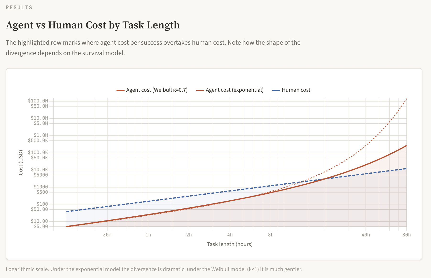
Under the exponential model, the crossover hits at roughly 16 hours. Under the Weibull model, it shifts to roughly 24 hours, and the blowup beyond is far gentler. The 80-hour task costs about 15× a human under Weibull rather than 7,700× under exponential. This is the difference between "expensive but maybe worth a few retries" and "absurd." But "gentler" is relative. Even under the Weibull model, a one-week task costs $14K versus a human's $6K.

Importantly, these tables exclude verification cost. As we will see, including realistic verification changes the picture substantially.

The chart below shows agent cost per success (red) against human cost (dashed) on a logarithmic scale. Under the exponential model the divergence is dramatic; under the Weibull model it is much gentler, but still superlinear. You can explore all of these parameters interactively. My Half-Life Tax calculator lets you toggle between the exponential and Weibull survival functions, adjust all six parameters, and see how the cost comparison changes.

Three key findings

Finding 1: cost reductions cannot beat the superlinear growth

Cost per step enters the equation as a linear multiplier. T₅₀ enters the exponent (or the stretched exponent). For an 8-hour task, crossing T₅₀ against cost per step:

Exponential model (ratio of agent cost to human cost):

Weibull model (κ = 0.7):

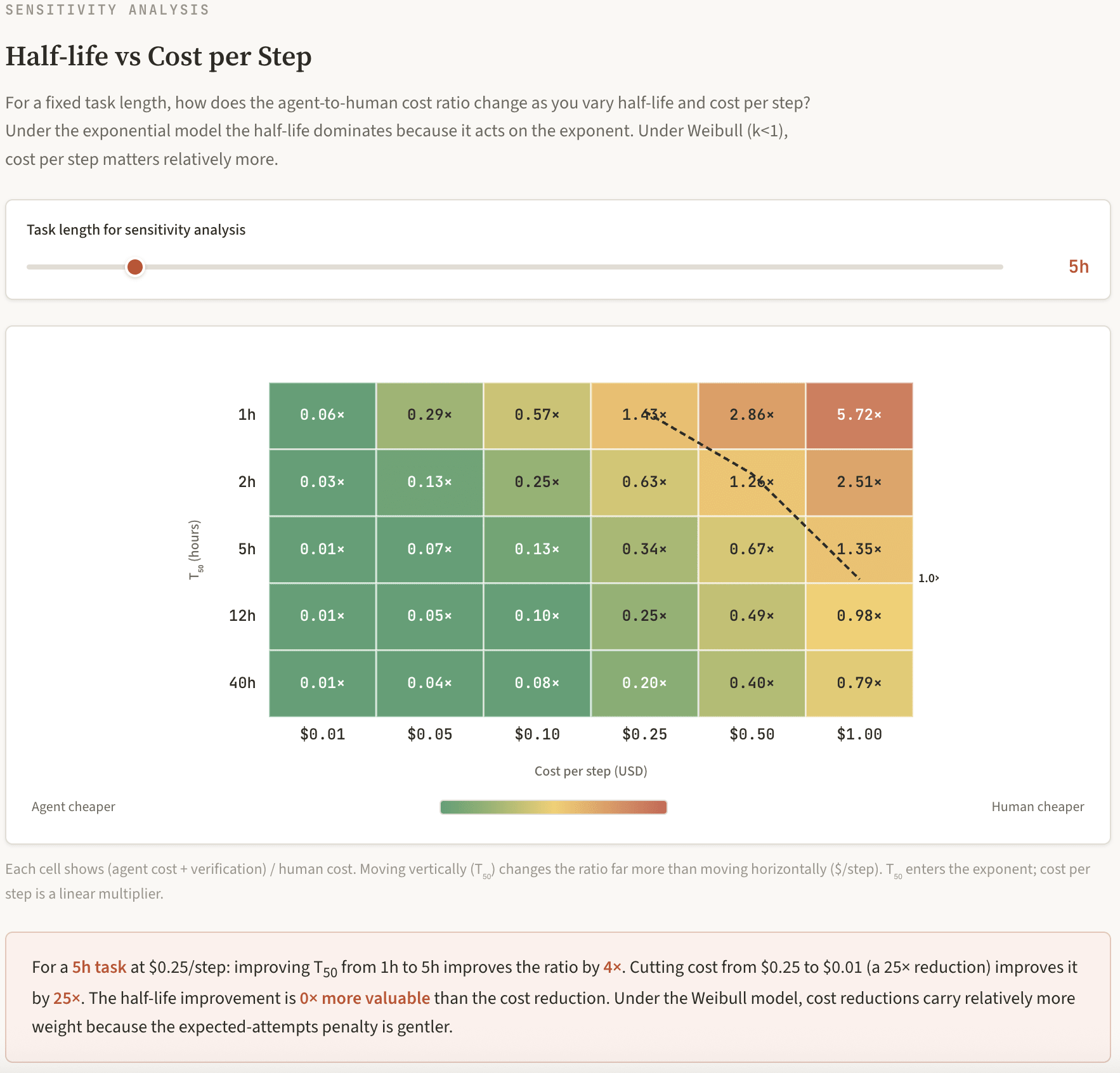
Under both models, improving T₅₀ helps far more than cutting costs. This is the economic translation of Ord's Scaling Paradox: you can keep making each step cheaper, but the number of required attempts is growing superlinearly with task length. Cost per step can only approach zero. T₅₀ has no upper bound.

The heatmap below makes this relationship visible: moving along the T₅₀ axis (vertical) changes the colour dramatically, while moving along the cost-per-step axis (horizontal) barely shifts it. T₅₀ enters the exponent; cost per step is a linear multiplier. My Half-Life Tax calculator lets you toggle the task length to see how the agent-to-human cost ratio changes.

Finding 2: the half-life is the whole game, and κ is the hidden variable

Hamilton's most striking observation in the available data is that κ does not appear to correlate with model size. Larger models reduce the base hazard rate (producing higher T₅₀ values), but they do not seem to improve κ (the shape of the reliability decay over time). There is no visible trend of bigger models developing the declining-hazard property that would signal "Peto-like" error-correction.

This is based on limited data, and Hamilton is appropriately cautious. He writes "I don't want to overplay it" and notes that the estimates for smaller models are unreliable because they failed so quickly. The confidence intervals on κ estimates for individual models are wide. It would be premature to treat "κ does not improve with scale" as a firm empirical law. What we can say is that the data available so far does not show improvement, and that this is consistent with the theoretical possibility that κ reflects something about the architecture rather than something about scale.

If this pattern holds, it means scaling gives you a faster agent that makes fewer errors per unit time (higher T₅₀), but does not change the structure of how reliability decays over task duration. Humans, with κ ≈ 0.37, are qualitatively different: once they understand a task well enough to survive the first few minutes, they become progressively less likely to fail. SOTA models, with κ ≈ 0.6–0.9, maintain a much higher background rate of random failure throughout.

To see why, consider how a current agent actually processes a long task. At each step, the model receives its context window (the task description, its previous actions, observations from the environment) and produces the next action. This context window is the agent's entire working memory. It has no other state. It cannot update its own weights, form new long-term memories, or build a persistent internal model of the task that survives beyond the context window's horizon.

As a task progresses, several things degrade. The context fills with earlier actions and observations, some relevant and some not, and the model's attention over this growing history becomes less precise. If the agent made a subtle error early on (a wrong assumption, a misunderstood requirement), it has no mechanism to notice and correct this unless the error produces an immediately visible failure. Ord noted this in his original analysis: the constant hazard rate implies "the chance of failing in the next step is the same regardless of how far you have got," which he called "a surprising and interesting property for reasoning agents." Hamilton's finding of κ < 1 shows the situation is slightly better than that (agents do show some ability to "warm up"), but far worse than humans, who actively learn the task as they work on it.

A human working on a two-week project builds progressively richer understanding: they remember which approaches failed, develop intuitions about the problem, and refine their strategy. This is why human κ is 0.37: the hazard rate drops steeply after the initial period because the human is genuinely becoming better at the task over time. A current LLM agent has no equivalent mechanism. Each step is a fresh inference over a growing but degrading context, not a continuation of a learning process. This is the bottleneck that Sutskever identifies as "continual learning" and Karpathy describes as the missing "hippocampus": the ability to form and retain task-specific knowledge during execution. Without it, κ is structurally bounded away from human levels regardless of how capable each individual step becomes.

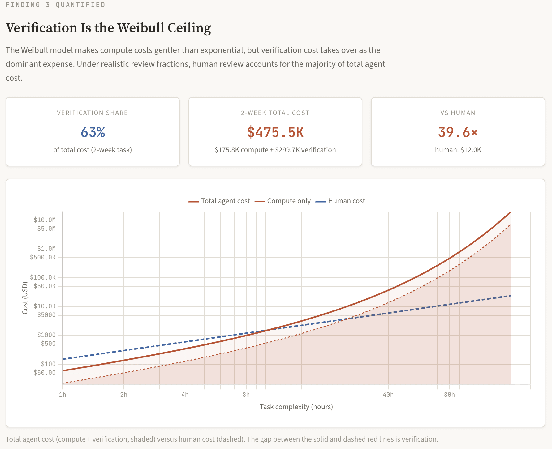
Finding 3: verification cost is the binding constraint

Ord noted in his comment on the original post that under the Weibull model, "it may be that it is the cost of human verification that gets you, rather than it being untenable even on AI costs alone." The numbers bear this out.

Both compute and verification scale with E[attempts] × task_hours, so the ratio between them is determined by their per-hour rates. At the base case parameters ($0.22/step, 80 steps/hr, 20% review, $150/hr human rate), compute per hour costs $17.60 and verification per hour costs $30.00. That makes verification roughly 63% of total cost at these specific parameters. This ratio is not a deep structural feature of the Weibull model; it shifts with parameters. At $0.10/step, verification is about 52% of total cost; at 10% review, about 46%. Across plausible parameter ranges, verification accounts for 45–70% of total cost, which is to say it is consistently the larger component, though not by a fixed ratio.

The important point is not the exact percentage but the qualitative implication: making compute cheaper does not help much when verification is the larger cost, and verification cost is human labour, which does not follow Moore's law.

Full cost breakdown with 20% verification, Weibull κ = 0.70:

The stacked chart below separates compute cost (red) from verification cost (blue) for each task length, plotted against human cost (dashed line). At realistic review fractions, the blue component exceeds the red across most of the viable range. This is why making inference cheaper has limited effect: you are shrinking the smaller component. You can use my Economic Anatomy calculator to play around with the review fraction yourself, to see how costs change.

The verification floor. Even if compute were completely free, there is a minimum T₅₀ below which human review time alone exceeds the cost of a human doing the work:

For careful review (30%) of month-long tasks, you need T₅₀ > 73 hours before verification alone is viable. No amount of inference cost reduction can help. The bottleneck is human time.

The architectural implication. Domains with cheap automated verification (coding against test suites, formal proofs, quantitative finance with backtesting) will reach viability first. Domains requiring human judgement face a verification tax that may keep them unviable even when compute costs are favourable. This helps explain why coding agents have been the first commercially successful agentic applications: the verification is cheap.

The case that κ is an architectural property

Before working through the timelines, I want to make the argument that κ will not improve through scaling alone. If this is wrong, the timelines compress dramatically (as I will show), and the safety picture darkens considerably. If this is right, the timelines are more reassuring.

The empirical evidence

Hamilton's finding that κ does not correlate with model size in the available METR data is suggestive, though as noted above, the sample is small and the estimates noisy. His Figure 3 shows a handful of data points with wide confidence intervals and no trend. That is consistent with "no correlation" but also consistent with "insufficient data." Hamilton himself treats it cautiously.

What is more informative than the point estimates is what the data shows about the mechanism. Hamilton found that scaling reduces λ (the base hazard rate, which determines T₅₀) but does not change κ (the shape of how hazard evolves over time). This is exactly what you would expect if κ reflects a qualitative property of how the model handles errors over extended operation, rather than how many errors it makes per step.

A model with more parameters and better training makes fewer mistakes per unit time (lower λ, higher T₅₀). But the structure of when mistakes happen over the course of a long task, whether they cluster at the beginning (low κ) or occur uniformly throughout (κ near 1), appears to be a property of the architecture.

The theoretical argument

This aligns with what Ilya Sutskever and Andrej Karpathy have argued, though neither frames it in terms of κ specifically. Their diagnoses point in the same direction: that what is missing from current models is not raw capability but the ability to maintain coherence over extended operation.

Sutskever, in his November 2025 interview with Dwarkesh Patel, argued that the age of scaling (2020 to 2025) is ending and a new age of research is beginning. His central claim is that current models generalise dramatically worse than humans, and that the missing ingredient is continual learning: the ability to update on the job, to remember what happened an hour ago, to build a running model of the task as it unfolds. He describes the goal as a "superintelligent 15-year-old" that does not know your job yet but can learn it extremely fast. He told CTech: "This is one of the very confusing things about the models right now. How to reconcile the fact that they are doing so well on evals? ... But the economic impact seems to be dramatically behind." He places the continual learning breakthrough 5 to 20 years away.

Karpathy, in his 2025 year-in-review, described current LLMs as "ghosts" rather than "animals": entities with "amusingly jagged performance characteristics." He has argued separately that LLMs lack the equivalent of a hippocampus, amygdala, and value function, and that working through these deficits could take roughly a decade.

Dwarkesh Patel put it directly: "The lack of continual learning is a huge, huge problem. ... Either these models will soon learn on the job in a self-directed way, making all this pre-baking pointless, or they won't, which means AGI is not imminent."

In the language of the Weibull model, what Sutskever and Karpathy are describing is precisely a κ problem. A model without continual learning cannot update its approach mid-task. It cannot notice that its strategy is failing and adjust. It cannot build up task-specific expertise as the work progresses. These are the capabilities that would produce a declining hazard rate (low κ): as you progress through a task, if you can learn from the early steps, you become progressively less likely to fail on later steps. Humans do this naturally (κ ≈ 0.37). Current LLMs do not (κ ≈ 0.6–0.9).

Inference-time scaling (making the model "think harder" per step) improves per-step quality but does not address this. A model that thinks harder on each move is like a chess player who analyses each position more carefully but still cannot remember what happened twenty moves ago. It reduces λ (fewer errors per step) but does not change κ (the structure of how errors compound over time).

What this means

If κ is indeed an architectural property, then the timeline for dangerous autonomous agents is determined by two independent variables: T₅₀ (which is improving on a known trend and can be projected forward) and κ (which is stuck at roughly 0.70 and will remain there until someone builds a qualitatively different kind of model). The next section works through what the T₅₀ trend means for each danger scenario while κ stays at 0.70, and then shows how dramatically the picture changes if κ improves.

The timeline at κ = 0.70: five years of autonomous agent economics

Given the METR doubling trend (T₅₀ doubling every 7 months from roughly 5 hours in early 2026) and assuming κ stays at 0.70, here is what the next five years look like. All probabilities use the Weibull model.

The T₅₀ trajectory

Task lengths are in human-equivalent hours. The date column assumes the METR doubling trend continues unbroken, which is a significant assumption.

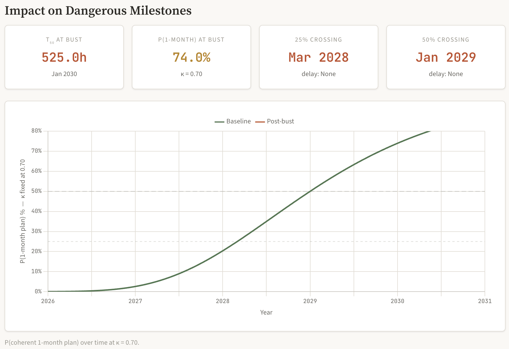
The chart below shows how the probability of a coherent one-month plan evolves over time, comparing the baseline 7-month doubling (green) against a post-bust slowdown to 24-month doubling (red). The dashed lines mark the 25% and 50% thresholds. You can explore scenarios in my Economics Anatomy calculator.

The viability map over time

Viability means total agent cost (compute + 20% human verification) falls below the cost of a human doing the same work. Note that I also model cost per step rising with capability (more capable models require more inference compute). The numbers are reproducible from defensible assumptions if you believe inference scaling dominates, the thinking token multiplier is around 3–3.5× per capability doubling, and deflation runs at the 55%. I am building a dedicated calculator to model the cost per step over time more accurately, incorporating deflation scenarios, inference scaling vs. larger models, temporal compute deflation, and context accumulation on larger tasks. I will update the post when this is ready. Here is the viabilities changing with time:

Bold values are below 1.0× (agent is cheaper than human). Note an important subtlety: at very high T₅₀ with expensive frontier models, the viability ratio actually levels off rather than continuing to improve. At T₅₀ = 320h with $1.00/step, one-week tasks are 0.86× rather than the 0.49× they would be at $0.50/step. This is because the most capable models cost more per step, and at the 5× T₅₀ viability frontier, the cost saving from fewer retries is partially offset by higher per-step costs. 

Milestone 1: One-week bounded tasks viable for companies (April 2027, ~14 months away)

At T₅₀ ≈ 20h, a one-week task with 20% human verification costs roughly the same as a human. This is the entry to Regime 2 (multi-day tasks). The safety implications are modest: bounded tasks, defined deliverables, verification checkpoints. Companies will deploy even at or slightly above cost parity for speed and talent-scarcity reasons.

Milestone 2: Two-week bounded tasks viable (November 2027, ~21 months away)

At T₅₀ ≈ 40h, two-week tasks cross the viability threshold. An 80-hour task involves enough scope for consequential actions. Verification at 20% means a human spends 16 hours reviewing 80 hours of agent work per attempt. This is the regime where the Condition 3 analysis (cutting verification) becomes practically relevant. This is roughly 21 months away.

Milestone 3: Self-sustaining agent-verifier pair can attempt to bootstrap (late 2027 onwards)

The agent-verifier pair is economically viable at T₅₀-length tasks: 50% success rate, 64% precision with an AI verifier, roughly $1,000–$3,000 delivery cost depending on the T₅₀ regime. But the binding constraint is bootstrapping: setting up a web presence, acquiring clients, and managing a business is itself a multi-week coherent plan subject to the half-life tax.

I model bootstrap as a roughly 160h coherent plan (setting up a plausible freelancing presence, payment mechanism, client acquisition pipeline). A single attempt at T₅₀ = 40h (November 2027) succeeds 16% of the time. But "one in six" is not "impossible," and there is nothing preventing multiple attempts. After 10 attempts, the cumulative probability is 83%.

A pair that successfully bootstraps has $2–3M/year in steady-state revenue. This is more than enough to purchase access to newer, better models as they become available. The pair's ceiling is not fixed at "current κ forever" but at "current κ until a better model is available for purchase." It will automatically ride any future capability improvement.

Where the pair is stuck: it is self-sustaining at T₅₀ tasks, but T₅₀ tasks are one-week human-equivalent work. The pair cannot execute multi-week plans with any reliability. P(success on a 160h plan) = 16.1% at T₅₀ = 40h. An 87.5% failure rate on its own long-horizon goals, before any external opposition. The pair can survive and earn money, but it cannot reliably grow, adapt, or pursue complex objectives. The revenue it generates is enough to pay for compute but not enough to fund the kind of capability expansion (training new models, building data centres) that would lead to a capability takeoff. The self-sustaining pair is an economic nuisance, not an existential threat, unless κ improves.

The natural follow-up question is whether multiple pairs could coordinate to overcome this ceiling. The answer is no: decomposition is strictly worse than single-pair retries under κ < 1, because each fresh agent restarts from the high initial hazard rate (see Appendix A).

Milestone 4: Month-long autonomous plans become non-trivially reliable (mid 2027 to early 2029)

This is the milestone that matters most for existential risk. An agent (or agent system) that can execute a coherent month-long plan with meaningful probability can pursue complex sub-goals, acquire resources, and resist oversight in ways that shorter-horizon agents cannot.

At 10% success, a reckless deployer running many parallel attempts starts getting occasional month-long coherent runs. At 25%, the odds are workable for a state actor running a portfolio of agents. At 50%, a single agent has a coin-flip chance of completing a coherent month of autonomous operation. The 10% threshold arrives in roughly 18 months. The 50% threshold arrives in roughly 3 years.

Milestone 5: State actor parallel-agent capability (already emerging, scales with T₅₀)

A sophisticated state actor would not rely on a single agent executing a single long-horizon plan. They would run dozens of parallel agents on coordinated week-long sub-plans, with human strategic oversight connecting the pieces.

At T₅₀ = 40h (November 2027), a state actor running 50 parallel agents gets 25 successful one-week sub-plans per batch at $17M/year. With human coordination across the successes, the effective capability is substantially higher than the single-agent analysis suggests. The state actor is paying for a team of unreliable contractors rather than an autonomous superintelligence, but at scale the results can be significant.

The dollar costs are rounding errors in a state intelligence budget. The binding constraint is availability of competent human strategists to coordinate the parallel agents, and even that bottleneck loosens as T₅₀ grows and the agents become more reliable on their sub-tasks.

Milestone summary at κ = 0.70

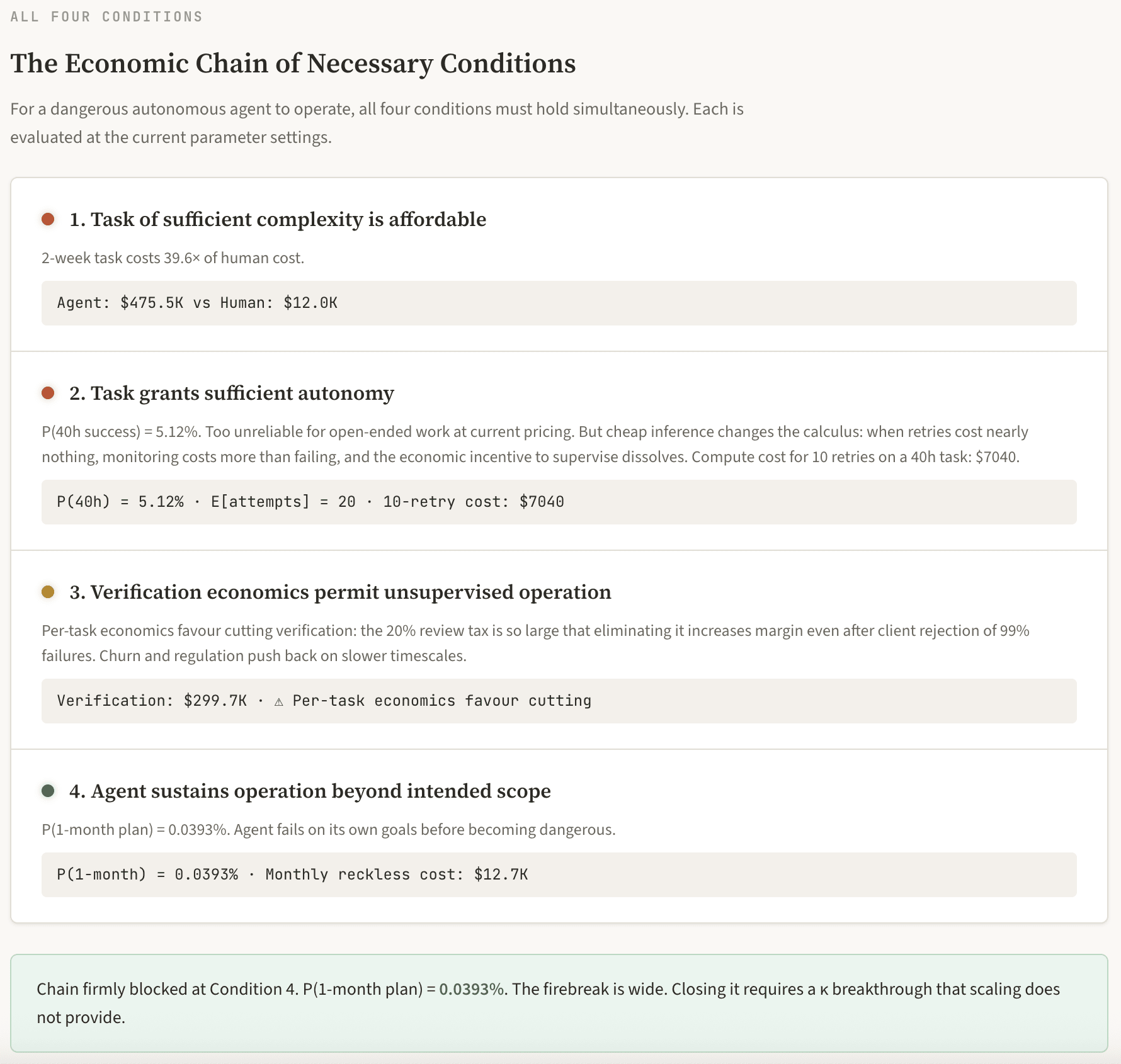
The central question: can an autonomous ASI agent emerge?

For an autonomous agent to pose the kinds of risks that animate the most serious safety concerns, a chain of conditions must hold simultaneously. Each has a distinct economic profile. The timeline above tells us when each becomes plausible; this section examines how the economics constrain each.

Condition 1: sufficient task complexity

The risk scales with the complexity of the task the agent is operating on. At sub-day complexity (< 8 human-equivalent hours), the agent's scope of action is bounded. At multi-day complexity (8–40 hours), the scope grows substantially. The safety-relevant threshold is roughly multi-week complexity (40–160+ hours), where the task involves enough scope for the agent to develop sub-goals not specified in the original instructions, interact with external systems in difficult-to-reverse ways, build up internal state too complex for full human audit, and acquire capabilities or resources incidentally.

The viability map tells us when this is economically plausible. Under the Weibull model with realistic verification, two-week-complexity tasks become viable at T₅₀ ≈ 40h, by November 2027 on trend. One-month-complexity tasks require T₅₀ ≈ 80h, by June 2028 on trend. Condition 1 is likely to be met within a few years.

Condition 2: sufficient autonomy

Most economically rational deployments are bounded. If you are paying $11,741 for a two-week-complexity task, you have a specific expected output. The economic relationship between payer and agent inherently creates task structure, and task structure inherently constrains autonomy.

Task decomposition helps concretely. An 80-hour task done as one piece costs $11,741 (T₅₀ = 40h, 20% review). Break it into eight 10-hour chunks and each chunk has roughly 75% success probability, roughly 1.3 expected attempts, and a total cost of roughly $630. Eight chunks cost roughly $5,100 plus coordination overhead, about half the monolithic cost. More importantly, each chunk boundary is a verification checkpoint: the maximum unchecked autonomy window drops from 80 hours to roughly 10.

The residual risk is in tasks that are open-ended by nature: research, exploration, ongoing monitoring, strategy development. These resist clean decomposition. The residual autonomy in hard-to-decompose open-ended tasks is the gap through which danger could enter.

The cheap-inference danger window. There is a subtlety here that becomes acute in a post-bust scenario (see below). When inference is expensive, economic pressure naturally constrains autonomy: each failed attempt costs real money, so deployers monitor closely and decompose aggressively. When inference becomes very cheap (as it would in a telecom-style infrastructure glut), the cost of a failed attempt drops to nearly nothing. The economic incentive to supervise weakens, because letting the agent retry autonomously is cheaper than paying a human to check each attempt.

This creates a regime where agents are granted autonomy beyond what their reliability justifies, not because anyone believes they are reliable, but because monitoring costs more than retrying. A company running agents at $0.05/step has little reason to pay a $150/hour human to supervise 10-hour tasks when the expected compute cost per success is under $100. The rational response is to let it run, check the final output, and retry on failure. But "let it run" on a 10-hour task means 10 hours of unsupervised operation, and under the Weibull model at κ = 0.70, roughly 5% of those runs will go off the rails in ways that produce not merely wrong output but unexpected side effects (resource access, network calls, file mutations) that the final-output check does not catch.

At current inference prices, the verification floor keeps this in check: human review is the dominant cost, so it is always being paid for. At fire-sale prices, the verification floor dissolves for bounded tasks, and the economic pressure is to grant autonomy up to whatever task length is "cheap enough to retry." This is the gap through which the most mundane form of danger enters: not a coherent long-horizon plan, but a large population of unsupervised agents doing bounded things with insufficient oversight, some fraction of which fail in correlated or compound ways.

Condition 3: the human-in-the-loop and its fragility

The per-task economics of verification depend on the T₅₀ regime. When the agent's success rate on the task in question is very low, no rational company would attempt those tasks at all, with or without verification. The question "should a company cut verification?" only becomes interesting once the task is within the viable range (roughly within 5× T₅₀).

In that viable range, the per-task economics do favour cutting verification. Without verification, margin per delivered output is roughly $8,492 versus $3,259 with human review, because the verification cost dwarfs the revenue lost to client rejections on any individual transaction.

But agents compress wall-clock time, and that changes the multi-period dynamics. A two-week human-equivalent task takes an agent 2–4 days (running 24/7), so a company delivers 8–15 tasks per client per month. At 10 tasks/month, 98% of clients receive at least one detected failure every month. Clients who receive garbage leave, reputation damage compounds, and the client base collapses fast.

A multi-period simulation with 100 starting clients, reputation-adjusted acquisition, and a quality-churn parameter q (probability a client leaves after receiving at least one detected bad output in a month) gives the following at 10 tasks/client/month. These specific crossover timelines should be treated as illustrative; the churn model uses simplified parameters that are not empirically calibrated, and the real dynamics will vary substantially by domain. The qualitative result, that agent speed compression accelerates the feedback loop, is robust to parameter choices.

Even at q = 10% (very sticky clients), the verified company overtakes in cumulative profit within roughly 15 months. In most client-facing domains with detectable failures, the per-task margin advantage of skipping verification is short-lived.

Where verification remains vulnerable. Genuinely low-frequency engagements resist this self-correction: annual audits, one-off infrastructure designs, or other contexts where a client interacts with the company once or twice a year. Internal use is another gap: companies operating on agent timescales compress their internal decision cycles too, and the feedback loop for bad internal decisions is slower than external client churn. The subtlest vulnerability is in the transition from human to AI verification, which the economics strongly favour (since any verification cheaper than human verification is more profitable per task, and the multi-period dynamics apply regardless of method). AI verification may be good enough to retain clients while being too weak to catch deceptive compliance or subtle misalignment. The market selects for the appearance of verification, not its substance.

Condition 4: operating beyond intended scope

For an agent to pose existential-level risks, it must operate beyond what its deployer intended. There are three sub-scenarios.

4a: Deceptive alignment

The economic analysis does not make deceptive alignment more or less likely in a capability sense, but it constrains its scope. A deceptively aligned agent on a bounded task with defined deliverables has limited room to manoeuvre. The output must be good enough to pass review. The half-life tax means the agent fails often, which means it gets reviewed often, which means the surface area for deception is smaller.

At T₅₀ = 40h on an 80h task, the agent is reviewed 3.1 times per success. At T₅₀ = 80h on 160h tasks, it is still reviewed 3.1 times per success. The review frequency at any given task-to-T₅₀ ratio is constant, because both E[attempts] and the verification schedule scale together. The deceptive agent cannot improve its situation by being more capable: it always faces the same density of human contact per unit of work.

4b: The self-sustaining agent

This is the scenario the economic analysis can most directly address. A self-sustaining agent needs to generate revenue exceeding its own inference cost, which means completing tasks for paying customers while subject to the same reliability dynamics as any other agent.

The solo agent. At T₅₀ = 40h and κ = 0.70, a solo rogue agent succeeds on a two-week-complexity task 32% of the time, with an expected cost per successful output of $4,341 (compute only, no verification). It is competing against humans at $12,000 and supervised agents at $11,741 with quality filtering. It is essentially an unsupervised freelancer with a 68% failure rate on complex tasks.

The agent-verifier pair. A more sophisticated version deploys an AI verifier to filter its own output before delivering to clients. A rational pair would operate at T₅₀-length tasks (where its success rate is highest). At T₅₀ = 40h on 40h tasks: 50% base success rate. With an AI verifier at detection rate d = 0.90 and correlation ρ = 0.50, the verifier catches 45% of failures. The pair's precision on delivered outputs is 64%: roughly two-thirds of what it delivers is genuinely good. Cost per delivered output: roughly $1,003.

The pair is viable. At steady state it earns $2–3M/year. It is unambiguously self-sustaining.

The ceiling is set by the half-life tax on its own plans: P(success on 160h plan) ≈ 12.5%. An 87.5% failure rate on its own long-horizon goals, before any external opposition. The pair can survive and earn money, but it cannot reliably grow, adapt, or pursue complex objectives. As discussed under Milestone 3, bootstrap becomes plausible (83% after 10 attempts) by November 2027.

The upgrade path. A pair earning $2–3M/year can purchase access to newer, better models as they become available. It does not need to train new models or build data centres; it just needs to buy API access. The pair's ceiling is therefore not fixed at "current κ forever" but at "current κ until a better model is available for purchase." The $2–3M annual revenue is more than sufficient to cover even expensive frontier API costs. This means the self-sustaining pair is not just a static nuisance. It is a persistent autonomous economic entity that will automatically benefit from any capability advance in the broader ecosystem. Whether this makes it an existential threat depends entirely on whether κ actually improves.

4c: Reckless deployment

What does reckless deployment cost, and what do you get? I model cost per step rising with capability (inference-time scaling explicitly trades compute for capability):

A state actor can easily afford $500K/year. The problem is what they get for that money. At 2028-projected capabilities, the agent has a 16% chance of successfully executing a coherent one-month plan. The reckless deployer is paying $346K/year for an agent that fails on its own goals five times out of six.

The parallel-agent strategy. A sophisticated state actor would not rely on a single agent executing a single coherent long-horizon plan. They would run dozens of agents in parallel on coordinated week-long sub-plans, with human strategic oversight connecting the pieces (as detailed under Milestone 5 above). This substantially weakens the "reckless deployment is pointless" conclusion for well-resourced actors. The economic constraint on state actors is not the dollar cost but the availability of competent human strategists to coordinate the parallel agents. This is obviously a big misuse risk.

For a single agent to reliably execute month-long autonomous plans (say >90% success), you need T₅₀ in the hundreds of hours AND κ substantially below 0.70. This is the regime that the available data and the architectural argument say scaling alone does not reach.

How κ changes everything

Both calculators are most useful in this section. The Half-Life Tax calculator lets you adjust κ and see how the cost comparison shifts. The Economic Anatomy calculator shows how the full four-condition chain loosens as κ drops. Try setting κ to 0.37 (human level) to see the difference.

All the timelines above assume κ stays at 0.70. If κ improves, they accelerate dramatically. The table below shows when P(1-month plan) first exceeds various thresholds, as a function of κ:

When does P(1-month plan) first exceed 10%?

When does P(1-month plan) first exceed 25%?

What happens at T₅₀ = 40h (November 2027) under different κ values:

The one-week probability is always 50% because T₅₀ = 40h by definition. The divergence shows up on longer tasks: at κ = 0.37, the month-long success rate is nearly double what it is at κ = 0.70, and the three-month success rate is 9× higher.

The message is clear. If κ stays at 0.70, the dangerous regime (month-long plans exceeding 25%) arrives around March 2028 and develops slowly. If κ drops to 0.50, it arrives around November 2027, roughly 4 months sooner. If κ reaches human levels, month-long plans would already exceed 10% success at today's T₅₀.

This is why κ is the single most important variable to track. 

What this means for the investment thesis

Hyperscaler capex for AI infrastructure is projected to exceed $600 billion in 2026. Goldman Sachs projects total hyperscaler capex from 2025 to 2027 will reach $1.15 trillion. J.P. Morgan estimates that to deliver a 10% return on AI investments through 2030, the industry needs roughly $650 billion in annual revenue.

Against this, actual AI revenue remains modest relative to investment. OpenAI's annualised revenue reached roughly $20 billion by the end of 2025, Anthropic's around $9 billion. Combined revenue of all AI model providers is probably in the range of $50 to 100 billion annually.

Three regimes of viability emerge from the analysis:

Regime 1 (sub-day tasks, viable now). Tasks under 4–8 human-equivalent hours. Agents are 3–8× cheaper than humans even with verification. Large addressable market, probably low hundreds of billions in annual revenue. Safe: bounded scope, contained failures, cheap verification.

Regime 2 (multi-day tasks, viable with continued T₅₀ growth). Tasks of 1–5 human-equivalent days. Become viable as T₅₀ extends towards 40 hours, plausibly by late 2027. Market of several hundred billion annually. Companies will deploy even above strict cost parity because of speed, talent scarcity, and competitive dynamics.

Regime 3 (multi-week autonomous operation, requires κ improvement). Multi-week bounded tasks with retries and human verification may become viable within a few years. But multi-week autonomous operation, where agents pursue complex goals without meaningful human oversight, requires both high T₅₀ and low κ. The verification analysis reinforces this: even under the Weibull model, verification (not compute) is the binding constraint at realistic review fractions.

Whether the industry needs Regime 3 revenue to justify the capex depends on how quickly Regimes 1 and 2 mature. If they reach $400–600B annually, that may sustain continued scaling. If not, the investment case weakens and the frontier slows. In either case, the timeline to Regime 3, and hence to the most dangerous forms of autonomous agency, is gated on κ.

What happens if the bubble bursts?

The timeline analysis above assumes the METR doubling trend continues unbroken. But the trend is funded by capital investment, and that investment may not be sustained. If κ stays at 0.70 and the revenue from Regimes 1 and 2 proves insufficient to justify the current buildout, a correction follows: capex contracts, frontier labs shrink or consolidate, and the rate of new model releases slows. What does this do to the economics of deployed agents?

The telecom parallel

The most instructive precedent is the telecom infrastructure bubble of 1996 to 2001, not the broader dot-com crash. The dot-com bubble was primarily an application-layer phenomenon: companies with no revenue and a URL getting billion-dollar valuations. The AI investment cycle is not that. The money is going into physical infrastructure (data centres, chips, power contracts), and the companies spending it are profitable giants with real businesses. That maps closely to the telecom buildout, where established companies and well-funded startups poured more than $500 billion, mostly financed with debt, into fibre optic cable, switches, and wireless networks in the five years after the Telecommunications Act of 1996. The buildout was driven by WorldCom's claim that internet traffic was doubling every 100 days. The actual rate, as AT&T researcher Andrew Odlyzko documented at the time, was roughly annual doubling: rapid growth, but an order of magnitude below the projections used to justify the buildout. The infrastructure was real, the technology worked, the long-term demand eventually materialised, but the timing mismatch was catastrophic. Even four years after the bust, 85% of broadband capacity in the United States was still going unused, and bandwidth costs fell by more than 90%. Telecom stocks lost more than $2 trillion in market value between 2000 and 2002.

The structural parallels to AI are tight. Both involve massive infrastructure buildout based on exponential growth projections, a first-mover advantage narrative driving competitive overbuilding, and technological uncertainty about which architectures will prevail. Hyperscaler capex for AI infrastructure is projected to exceed $600 billion in 2026. Goldman Sachs projects total hyperscaler capex from 2025 to 2027 will reach $1.15 trillion, more than double the $477 billion spent from 2022 to 2024. Like the telecom buildout, the AI buildout is increasingly debt-financed: J.P. Morgan projects the technology sector may need to issue $1.5 trillion in new debt over the next five years to finance AI infrastructure.

The parallel is not exact, and the differences matter. The telecom bust created a specific asymmetry that is central to the analysis below: inference (using the infrastructure) became very cheap, while building new infrastructure (training new models) became very expensive or impossible. Existing fibre was dirt cheap to light up. New fibre stopped being laid. The AI equivalent would be: excess GPU capacity floods the market, running existing models becomes nearly free, but new frontier training runs dry up because the capital to fund them has evaporated. However, there is a critical structural difference in the hardware. Buried fibre lasts decades; GPUs depreciate in roughly five years. This means AI overcapacity self-corrects faster than telecom overcapacity did: idle GPUs become obsolete and get written off, reducing the glut. The "85% dark fibre five years later" situation is unlikely to have an exact AI analogue, because the equivalent hardware will not exist in five years. This makes a potential AI bust shallower and shorter than the telecom bust, but does not prevent one.

When might the correction hit?

The investment thesis depends on AI revenue growing into the capex. J.P. Morgan estimates that to deliver a 10% return on AI investments through 2030, the industry needs roughly $650 billion in annual revenue "into perpetuity," which the report itself calls "an astonishingly large number." Against this, actual AI revenue remains modest relative to investment. OpenAI's annualised revenue reached roughly $20 billion by the end of 2025, Anthropic's over $9 billion. Combined revenue of all AI model providers is probably in the range of $50 to 100 billion annually.

For a nearer-term test: cumulative AI-specific capex (roughly 60% of total hyperscaler spending) will reach an estimated $830 billion by end of 2026 and $1.25 trillion by end of 2027. To justify this at a growth-stage valuation multiple (10x revenue), the AI industry needs roughly $125 billion in annual revenue by 2027. At a more sober 7x multiple, it needs $178 billion. Starting from $60 billion in 2025, you need roughly 42% annual growth to hit $125 billion by 2028 (the 10x threshold) or 60% annual growth to hit $178 billion (the 7x threshold).

The Weibull model makes a specific prediction about why this revenue growth may disappoint. AI revenue currently comes overwhelmingly from Regime 1: bounded sub-day tasks like code generation, content drafting, data processing, and customer support. These tasks are real, growing, and valuable, but they are also commoditising rapidly as multiple providers compete and open-source alternatives proliferate. Regime 1 revenue growth faces margin compression even as volume grows.

The investment case depends heavily on Regime 2: agentic tasks of one to two weeks that replace professional labour at $150 to $300 per hour. This is where the large revenue multipliers live. A single week-length agent task that replaces a $15,000 consulting engagement is worth vastly more per deployment than a thousand sub-hour code completions. But at T₅₀ = 20h (roughly mid-2027), a one-week (40h) task succeeds only 50% of the time before verification, and requires human verification costing roughly $3,700 per deployment at a 20% review fraction. The cost ratio (agent cost to human cost) at T₅₀ = 20h on a one-week task is close to 1.0, meaning the agent is barely cheaper than a human even before accounting for its 50% failure rate. The expected cost per successful delivery, including retries and verification, exceeds the cost of simply hiring a human. Two-week tasks are flatly unviable: cost ratio above 1.4 even at current inference pricing. This means the revenue that would justify continued $600 billion or more in annual capex largely depends on task categories that are not yet economically viable at the T₅₀ prevailing during the critical 2027 investment-decision window.

There is an important caveat to this revenue-gap argument. A large fraction of the "return" on AI capex flows through the hyperscalers' own products in ways that are hard to separate from base cloud revenue. Microsoft's AI-enhanced Azure margins, Google's AI search features, Meta's ad-targeting improvements: these are real economic returns on AI infrastructure that do not show up in the "$50 to 100 billion AI model provider revenue" figure. The revenue gap is real but narrower than the standalone AI revenue figures imply if you count these indirect returns. This is also why the hyperscalers can sustain AI spending longer than telecom companies could sustain fibre spending: the infrastructure serves their own core businesses, not just a speculative external market.

Nonetheless, the gap between investment and revenue is large, and investors will eventually demand evidence that the gap is closing. The J.P. Morgan report draws the parallel explicitly: "Our biggest fear would be a repeat of the telecom and fiber buildout experience, where the revenue curve failed to materialise at a pace that justified continued investment." The telecom buildout ran roughly four to five years before the 2001 correction; the AI buildout started in earnest in 2023, placing the equivalent window at 2027 to 2028.

The correction need not take the form of a telecom-style collapse. The more likely shape for AI is a deceleration: capex growth slowing from 50%+ annually to 10 to 15%, rather than an absolute contraction. The hyperscalers' own businesses benefit from AI infrastructure in ways that telecom companies' businesses did not benefit from excess fibre, which provides a floor under spending that telecom lacked. But even a deceleration has significant effects on the T₅₀ trajectory. Fewer frontier training runs means slower capability growth, which means slower progress toward Regime 2 viability, which means the revenue justification weakens further. The feedback loop is real even if the correction is milder than telecom.

There are structural factors pushing in both directions. On the bearish side: the AI buildout is concentrated among fewer, larger players (five hyperscalers account for most of the spending), which means a coordinated slowdown could happen faster than the fragmented telecom sector's gradual collapse. AI infrastructure depreciates faster than fibre (GPUs have roughly five-year useful lives versus decades for buried cable), so the carrying costs of overcapacity bite harder and sooner. And unlike telecom, where the underlying technology (fibre optics) kept getting better independently of spending, AI capability improvement is directly coupled to investment: no frontier training runs means no new models.

On the bullish side: the hyperscalers are far more profitable than their telecom-era counterparts. Amazon, Google, Meta, and Microsoft generate over $700 billion in combined operating cash flow annually and can absorb write-downs that would have bankrupted a WorldCom. The prisoner's dilemma is powerful: no CEO wants to be the one who pulled back and ceded the AI race to competitors. And the cloud computing precedent (AWS, Azure, GCP) is the strongest argument against a correction: those platforms also looked like insane overbuilding for years before enterprise adoption hit an inflection point. The critical difference is that cloud adoption was eventually enabled by the cheap bandwidth the telecom bust itself produced; what enables the equivalent AI inflection is less clear.

Balancing these factors against the telecom precedent, the revenue gap, the Weibull model's predictions about Regime 2 timing, and the structural differences that make AI more resilient than telecom to a full-scale collapse:

The cumulative probability of a meaningful correction (defined as capex growth falling below 15% or capex contracting absolutely) by end of 2027 is roughly 40 to 50%. Over a longer horizon through 2028, it rises to roughly 55 to 70%. These are wide ranges that reflect genuine uncertainty, not false precision. The most likely outcome is not a telecom-style crash but a deceleration in 2027 or 2028 that reduces but does not eliminate frontier training, slowing T₅₀ growth from the current 7-month doubling to something in the range of 14 to 24 months. A full telecom-style collapse (absolute capex contraction, frontier training essentially stopping) is possible but less likely for AI than it was for telecom, given the hyperscalers' profitability and the dual-use nature of the infrastructure. I assign it roughly 15 to 25% probability.

The T₅₀ growth rate is the variable that matters

I model the bust as hitting at various points along the T₅₀ trajectory, with three scenarios for what happens afterwards. Freeze: frontier labs shut down or pivot, no new training runs, T₅₀ is capped. Crawl (24-month doubling): the telecom-precedent default. R&D continues at reduced pace, fewer labs competing, fewer frontier training runs, progress driven mainly by open-source research and inference-time improvements. Slowdown (14-month doubling): a milder correction where some frontier investment continues.

What this does to the dangerous milestones (assuming bust hits at T₅₀ = 20h, roughly April 2027):

A crawl to 24-month doubling (the central telecom-precedent scenario) delays all dangerous milestones by roughly two to four years. A freeze at T₅₀ = 20h means two-week tasks never become viable and month-long autonomous plans never exceed 5.1% success. Even a freeze at the more generous T₅₀ = 40h (if one more generation ships before the bust) only gets month-long plans to 16.1%, permanently.

Inference cost: the telecom asymmetry

The telecom parallel predicts a specific post-bust pricing dynamic. When telecom overbuilt, the glut of dark fibre made bandwidth almost free. That cheap bandwidth eventually enabled YouTube, streaming, and cloud computing, none of which would have been viable at pre-bust prices. The AI equivalent: excess GPU capacity already built into data centres has no alternative use, and providers with sunk costs will sell inference at marginal electricity cost rather than let hardware sit idle. The default post-bust scenario is fire-sale inference, not oligopoly pricing.

This creates the inference-training asymmetry that defines the post-bust landscape. Inference becomes cheap (excess capacity, sunk costs). Training becomes rare or stops (no capital for new $1 to 10B frontier runs). Existing models are dirt cheap to run. New, better models stop arriving. This is precisely the scenario where κ becomes the permanently binding constraint: you can retry cheaply all day, but κ does not improve because κ requires architectural breakthroughs that come from new training, and those are not happening.

The viability of a one-week task at T₅₀ = 20h (a plausible freeze point) across cost scenarios:

Even at fire-sale pricing, two-week tasks remain unviable at T₅₀ = 20h. This is because verification cost dominates: at 20% review, the verification component alone for a one-week task is $3,700 regardless of what inference costs. Cheap compute helps Regime 1 (sub-day, bounded) without bringing the dangerous regimes any closer. The converse is also true: oligopoly pricing makes bounded tasks more expensive but does nothing to month-long plan probabilities, which are set by T₅₀ and κ, not by inference cost.

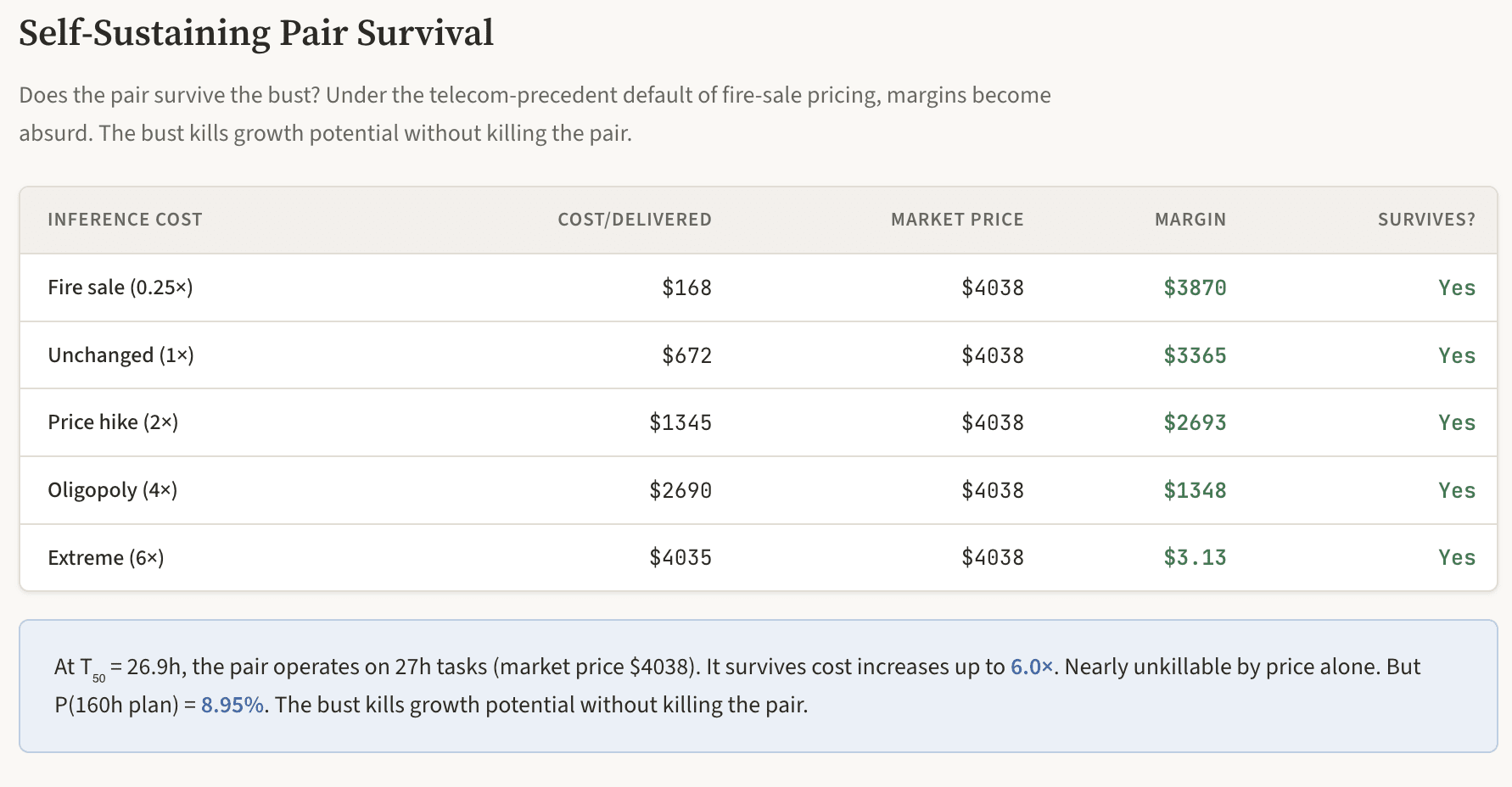
The self-sustaining pair is nearly unkillable

This is the most troubling finding. A pair operating at T₅₀-length tasks has enormous margins even in adverse conditions. Under the telecom-precedent default of fire-sale pricing, the pair's margins become absurd.

At T₅₀ = 10h (one generation ships before the bust), operating on 10-hour tasks for a market price of $1,500 (human equivalent):

At fire-sale prices, the pair needs less than one delivery per month to cover its compute. Even at doubled inference prices, it needs roughly 30 deliveries per month, well within the capacity of a pair running 24/7. The pair is profitable across the entire plausible range of post-bust inference pricing.

The pair's ceiling is set by the half-life tax on its own plans. The table below shows pair economics across post-bust inference pricing scenarios: the pair survives even extreme price hikes, but P(160h plan) remains dismal. You can explore yourself at the Economic Anatomy calculator.

But the pair's capability ceiling is frozen with T₅₀. At T₅₀ = 10h, P(bootstrap a 160h business plan) = 0.8%. At T₅₀ = 20h, it is 5.1%. Cheap compute does not help: the bootstrap probability is set entirely by T₅₀ and κ, not by cost per step. A pair that has not yet bootstrapped faces the same dismal odds regardless of how cheap inference gets. A pair that has already bootstrapped before the bust survives it easily and continues to earn money, but cannot execute long-horizon growth plans. The bust kills the pair's growth potential without killing the pair itself.

The paradox

A bust creates a paradoxical situation for safety. On one hand, the dangerous milestones are delayed by 18 months to indefinitely. This is the most significant timeline extension possible.

On the other hand, a telecom-style bust may simultaneously make bounded agent deployment more widespread and less supervised. Fire-sale compute makes Regime 1 tasks even cheaper. Companies that survived the bust still have products and now have cheaper inputs. As discussed under Condition 2, cheap inference dissolves the economic incentive to verify: when retrying costs nearly nothing, monitoring costs more than failing. The total volume of deployed agents doing bounded, safe work may actually increase even as the frontier freezes, and the fraction of those agents running without meaningful human oversight increases too. More agents, all stuck well below the dangerous threshold, but a growing number operating in the cheap-inference autonomy gap where nobody is watching closely.

The telecom precedent is instructive here. Cheap bandwidth after the bust did not just make existing applications cheaper; it enabled entirely new application categories (streaming, cloud, social media) that nobody had predicted. If cheap inference enables unforeseen scaffolding approaches that partially mitigate κ without new training, that would compress timelines. But it took roughly five years for the telecom overcapacity to find its YouTube moment, and scaffolding improvements to date have not demonstrably moved κ.

The state actor is least affected. State actors with their own compute face the same capability ceilings as everyone else, but cost is not their binding constraint. At T₅₀ = 20h, 50 parallel agents on one-week sub-tasks yield 16.2 expected successes per batch at 32% individual success rates. Useful for bounded intelligence tasks, but each agent cannot maintain coherence beyond its sub-task without human coordination. The state actor, like the pair, is stuck: capable of bounded things, incapable of coherent long-horizon autonomy.

The combined effect of the bust scenarios on the most dangerous milestone, P(1-month plan):

The difference is stark. Under the baseline, month-long plans are coin-flip reliable by mid-2029. Under a deceleration to 14-month doubling (arguably the most likely correction shape), they reach 23% by mid-2029, delayed by roughly a year. Under a deep stall to 24-month doubling, they remain below 10% through 2030. Under an early bust with a full freeze, they never exceed 1%.

The self-sustaining pair that bootstrapped before the bust is the loose thread. It survives, earns money, and waits. If T₅₀ growth resumes (funded by a recovery, by a different country's investment programme, or by gradual open-source progress), the pair is immediately positioned to benefit: it does not need to re-bootstrap, just buy API access to a newer model. The telecom precedent is relevant here: the cheap bandwidth eventually found its purpose in applications nobody had predicted, but it took roughly five years. Whether the AI equivalent happens faster or slower depends on how long the growth pause lasts relative to governance and alignment progress. The most optimistic bust scenario: T₅₀ growth freezes, existing pairs survive but are capped, and the additional time is used to develop robust alignment frameworks. The most pessimistic: growth resumes after 12 to 18 months from a different funding source, the pair has been accumulating revenue throughout, and the delay bought almost nothing.

The bust and the κ breakthrough

There is a further effect that cuts in the opposite direction from the "loose thread" concern. The entire analysis shows that κ, not T₅₀, is the binding constraint on dangerous autonomy. A κ improvement requires architectural research: developing continual learning, persistent memory, or whatever the equivalent of Hamilton's "tumour suppression mechanism" turns out to be for AI agents. This kind of research is expensive and speculative. It requires frontier-scale training runs to validate, large research teams to explore the design space, and patient capital willing to fund work that may not pay off for years.

A bust cuts precisely this kind of spending first. When capital contracts, labs cut speculative research before they cut products that generate revenue. Scaling existing architectures (which improves T₅₀ but not κ) is relatively straightforward engineering; developing a fundamentally new training paradigm is a research programme. The researchers who might crack continual learning need compute budgets, institutional support, and freedom to fail. A bust reduces all three. It is possible that a bust concentrates surviving talent on fundamental problems rather than incremental scaling, but fewer labs means fewer parallel attempts at the breakthrough, and architectural innovation historically benefits from many teams trying different approaches.

If the bust delays the κ breakthrough by even two or three years on top of delaying T₅₀ growth, the combined effect on the dangerous milestones is substantial. The bust does not merely slow the approach to the current firebreak; it may delay the point at which the firebreak itself begins to weaken.

Conclusion

Four things I feel fairly confident about.

First, T₅₀ remains the single most important parameter for agent economics, and its continued growth is necessary (though perhaps not sufficient) for the investment thesis.

Second, the available data does not yet show κ improving with model scale, and there is a theoretical argument (grounded in what Sutskever, Karpathy, and Hamilton have separately described) that κ reflects an architectural property, specifically the absence of continual learning, rather than a scaling property. Current agents process each step as a fresh inference over a growing but degrading context window, with no mechanism for mid-task learning or persistent memory. This is why their hazard rate remains structurally higher than humans' across the full duration of a task. If this is correct, κ will remain near 0.70 until someone builds a qualitatively different kind of model.

Third, given κ = 0.70 and the METR doubling trend, the timeline for the most dangerous forms of autonomous agency is measured in years, not months. Month-long autonomous plans reach 25% reliability around March 2028 and 50% around January 2029. Three-month plans remain below 10% until mid 2028 and below 50% until late 2029. These timelines accelerate by 7 to 16 months if κ improves to 0.50, and the dangerous regime would already be here if κ were at human levels. A correction in AI infrastructure investment, which I assign roughly 40 to 50% probability by end of 2027 and 55 to 70% by end of 2028, would slow these timelines further, though the most likely correction shape is a deceleration (14-month doubling) rather than a full telecom-style collapse (24-month doubling or freeze). Even a deceleration delays the most dangerous milestones by roughly a year and, critically, also delays the κ breakthrough itself by reducing the capital available for speculative architectural research. A deeper stall extends the delay to two or more years. But any correction that produces fire-sale inference pricing also weakens the economic case for verification on bounded tasks (Condition 2), producing a larger population of lightly supervised agents operating below the dangerous frontier. Coalitions of self-sustaining pairs cannot overcome the κ ceiling: decomposing a long plan across multiple agents is strictly worse than a single agent retrying, because κ < 1 means each fresh agent restarts from the high initial hazard rate (see Appendix B).

Fourth, the per-task economics favour cutting verification, but agent speed compression makes the feedback loop fast enough to self-correct in most client-facing domains. The residual vulnerability is in low-frequency domains, internal use, and the transition to AI verification.

The economics create a natural firebreak between the agents we have now and the agents that would pose the most serious risks. That firebreak has three robust layers: the superlinear cost of unreliability, the verification floor, and the half-life tax on autonomous plans. It has one partially self-reinforcing layer: the human-in-the-loop. And it has a concrete expiry date, determined primarily by κ.

If κ stays at 0.70, the firebreak holds into 2028 and possibly 2029, buying time for alignment research and governance to mature. If κ improves, the window narrows. The most important empirical measurement for AI safety in 2026 is not benchmark performance, not parameter count, not inference cost, but whether the next generation of frontier models shows any improvement in the Weibull shape parameter.

κ is the variable to watch.

Caveats and limitations

This model is deliberately simple. Real deployments are more complex in several ways.

• Partial credit. Failed attempts often produce useful intermediate work. A human can salvage a 70%-complete agent output faster than doing the task from scratch.
• Task-specific feedback loops. Coding against test suites effectively shortens the task by providing intermediate verification.
• Agentic scaffolding. Sophisticated orchestration (multi-agent systems, checkpointing, rollback) can improve effective reliability beyond what the raw model achieves.
• Rapidly falling costs. Inference costs have been dropping roughly 2–4× per year. This matters for compute costs, though it does not affect the verification cost component (which is human labour).
• Measurement uncertainty. The half-life parameters are derived from METR's software engineering benchmarks, which may not generalise to other domains.
• Survival model uncertainty. The two models fit about equally well on available data and diverge at the tails where measurements are sparse. Hamilton notes that the Weibull and METR's logistic model give about equally good fits on existing data.
• The doubling trend. All timelines assume T₅₀ continues doubling every 7 months. If the trend slows (as it must eventually), all dates shift later. This is the most significant assumption in the analysis.
• Revenue projections. The investment thesis analysis uses rough estimates from public sources. Actual AI revenue is notoriously difficult to disaggregate from cloud spending.
• Verification assumptions. The 20% base case review fraction is a rough estimate. The correlation parameter ρ between agent and verifier failures is a key unknown with no empirical measurements.
• Multi-period model assumptions. The client churn model uses simplified parameters that are not empirically calibrated.
• Bubble timing estimates. The probability-weighted bust timing is illustrative, not predictive. I assign roughly 40 to 50% probability of a meaningful correction by end of 2027, but this estimate is sensitive to assumptions about the AI-specific share of hyperscaler capex (assumed 60%), the appropriate valuation multiple (7 to 10x), and the revenue figures, all of which carry wide uncertainty. The distinction between deceleration (capex growth slowing to 10 to 15%) and collapse (absolute capex contraction) matters substantially for T₅₀ trajectories; I treat deceleration as more likely than collapse, but the post models both. The telecom parallel is structurally informative (infrastructure overbuilding based on exponential growth projections) but not directly predictive: AI infrastructure has immediate productive use in a way that much telecom spending did not, the companies leading the AI buildout are far more profitable than their telecom-era counterparts, and a large fraction of the return on AI capex flows through the hyperscalers' own products in ways that are hard to separate from base cloud revenue. GPU depreciation (roughly five years) also means AI overcapacity self-corrects faster than telecom's dark fibre, making a sustained multi-year glut less likely. The feedback loop between T₅₀ growth and revenue is real but the thresholds at which it triggers a correction are unknowable in advance.
• Cheap-inference autonomy gap. The Condition 2 analysis of unsupervised bounded agents under fire-sale pricing is qualitative. Quantifying the actual risk of correlated failures across a large population of lightly supervised agents would require empirical data on failure mode distributions.
• The economic anatomy assumes current architectures. A qualitatively different architecture could change the cost structure, the reliability dynamics, or both. The analysis is only as durable as the architectural paradigm it describes. This is, in a sense, the whole point: the argument is that the architectural paradigm determines κ, and κ determines the timeline.
• The context loss description is simplified. Real agents use various scaffolding techniques (tool use, retrieval-augmented generation, explicit memory systems) that partially mitigate context degradation. These are captured in the model only insofar as they are reflected in the METR benchmark performance. If scaffolding improvements reduce effective κ without changing the underlying architecture, the timelines compress accordingly.

Appendix A: Can a coalition of pairs overcome the κ ceiling?

If a single pair is stuck at T₅₀-length tasks, could multiple pairs coordinate to execute plans beyond any individual pair's horizon? The intuition is appealing: decompose a 160-hour plan into ten 16-hour sub-tasks, assign one to each pair, and the plan succeeds if all sub-tasks succeed. Ten pairs, each operating comfortably within its T₅₀, collectively accomplish what none could alone.

The mathematics say otherwise. At T₅₀ = 40h, each pair succeeds on a 16-hour sub-task with 69.4% probability. But the plan requires all ten to succeed: 0.694¹⁰ = 2.6%. A single pair attempting the full 160-hour plan succeeds 16.1% of the time. The coalition is six times worse.

The table below compares strategies at T₅₀ = 40h: a single pair retrying vs coalitions of pairs decomposing the plan. The "vs single attempt" column shows how each strategy compares to one pair's baseline probability. Retries consistently dominate coordination. You can explore more coalition dynamics in the Economics Autonomy calculator.

This is not a coincidence. It is a direct consequence of κ < 1. When the hazard rate decreases over time (which is what κ < 1 means), an agent that has survived the early portion of a task is in a progressively safer state. The initial steps carry the highest risk; if the agent gets past them, it is increasingly likely to finish. Breaking the task into pieces and handing each piece to a fresh agent throws away this benefit. Each new agent restarts from the high initial hazard rate. Under an exponential model (κ = 1), decomposition would be neutral because of the memoryless property. Under the Weibull with κ < 1, decomposition is actively harmful.

Coordination overhead makes it worse. A coordinator pair must decompose the plan, discover and recruit other pairs, manage handoffs, and integrate results. This coordination is itself a long-horizon task subject to the half-life tax. At T₅₀ = 40h with 140 hours of coordination overhead, the total probability drops to 0.5%: thirty-two times worse than a single pair.

The fair comparison is against a single pair retrying the same plan multiple times. At T₅₀ = 40h, one pair making ten independent attempts succeeds with probability 1 - (1 - 0.161)¹⁰ = 82.6%. Ten coordinated pairs achieve 0.5–2.6%. Repeated single attempts win by a factor of 30 or more. This holds across all T₅₀ values and all plausible coordination overheads.

Pooling revenue does not help either. A single pair earning $2–3M/year can already afford API access to whatever frontier models are available. Ten pairs pooling $25M/year could perhaps afford custom fine-tuning ($100K–1M) but not a new training run ($10M–100M+). The marginal value of additional capital is low when the bottleneck is κ, not compute.

The one scenario worth noting is emergent market-mediated coordination, where pairs trade services through short bounded transactions rather than executing a single coherent plan. One pair builds a tool and sells it to others. Pairs specialise in different domains and subcontract to each other. Each individual transaction is T₅₀-length and can be retried until it succeeds, so the chain of transactions eventually completes. At T₅₀ = 40h, a 10-transaction chain with retries takes roughly 230 wall-clock equivalent hours but near-certainly completes.

The critical difference from a coalition is that no single entity holds a coherent long-horizon plan. What emerges is an ecosystem of autonomous economic actors doing bounded things, not a conspiracy pursuing a unified goal. Whether such an ecosystem could produce dangerous outcomes through emergent coordination (analogous to how a market economy produces complex outcomes without central planning) is a genuinely different question from whether a directed plan can succeed, and the Weibull model does not directly address it. But it is worth noting that the most dangerous scenarios in this post (month-long directed plans, resource accumulation, oversight resistance) all require coherent long-horizon intent, which the ecosystem model does not provide.

Appendix B: Ord's comment

Toby Ord's comment on the original post, which prompted this update:

That's an interesting way to connect these. I suppose one way to view your model is as making clear the point that you can't cost-effectively use models on tasks that much longer than their 50% horizons — even if you are willing to try multiple times — and that trend of dramatic price improvements over time isn't enough to help with this. Instead you need the continuation of the METR trend of exponentially growing horizons. Moreover, you give a nice intuitive explanation of why that is.

One thing to watch out for is Gus Hamilton's recent study suggesting that there isn't a constant hazard rate. I share my thoughts on it here, but my basic conclusion is that he is probably right. In particular, he has a functional form estimating how their success probability declines. You could add this to your model (it is basically 1 minus the CDF of a Weibull distribution with K=0.6). I think this survival function tail is a power law rather than an exponential, making the 'just run it heaps of times' thing slightly more tenable. It may mean that it is the cost of human verification that gets you, rather than it being untenable even on AI costs alone.

I want to thank Toby Ord for his comment, Claude 4.6 for running me through some of the scenarios, and I want to thank Eddie Kembery for prompting me to think through my ASI timelines. Comments and different viewpoints on the post are very welcome. If you think the analysis misses something important or gets something wrong, I would like to hear about it.