Comments
Thanks for the post, and welcome to the EA Forum, Adam!
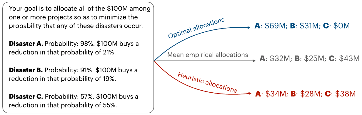
our results suggest that an extremely natural and seemingly obvious practice – presenting risk mitigation options individually for comparison – is suboptimal. Put bluntly: while people are relatively good at choosing individual items for their grocery carts given each item’s price per ounce (a linear allocation problem), people are less good at the nonlinear allocation problem of choosing individual existential risk interventions based on each intervention’s risk reduction per dollar spent. As a result, it may be better to instead present decision makers with competing total allocation profiles (specifying how much is to be invested in each risk), where each profile is explicitly labeled with its estimated reduction in overall existential risk (the risk that any catastrophe occurs).
The initial probability of survival in your example is (1 - 0.98)*(1 - 0.91)*(1 - 0.57) = 0.0774 %, which is pretty low[1]. In contrast, I think the probability of surviving human extinction nearterm is close to 100 %, with all potential causes being very unlikely to lead to it. So I would estimate the increase in the probability of surviving human extinction adding the decrease in the probability of each potential cause (because the other terms with multiple factors are much smaller). For example, "decrease in the probability of A" + "decrease in the probability of B" + "decrease in the probability of C", which is a linear allocation. As a result, neglecting diminishing returns decreasing each risk in isolation (as I think you assume), I would decrease the risk of human extinction spending all the money decreasing the risk for which "reduction in the risk of human extinction in pp"/"cost" is the highest.

Interesting piece! Good to see you on the forum, Prof. Elga -- I've read a lot of your work!
Thanks!