tl;dr

AI career advice orgs, prominently 80,000 Hours, encourage career moves into AI safety roles, including mid‑career pivots. I analyse the quality of this advice from the private satisfaction, public-good, and counterfactual equilibrium perspectives, and learn the following things:

1. Rational Failure: If you value personal, direct impact highly, it can be rational to attempt a pivot that will probably fail (e.g., $\ll 50\%$ success chance).
2. Misalignment: The optimal success rate for the field (maximizing total impact) often differs from the optimal rate for individuals (maximizing personal EV). The advice ecosystem appears calibrated to neither.
3. Counterfactual impact: Counterfactually, the value of a pivot can be lower than naïvely; in highly contested roles you need not only to be the best but to be the best by a wide enough margin to justify all the effort, and career pivots are negative EV for many plausible parameter ranges
4. Donations: If the EV of a pivot is uncertain, donating the attempt costs (e.g., the sabbatical expenses you were willing to pay) provides a guaranteed positive counterfactual impact.
5. Opacity: if we needed to work out whether our advice was producing good or not, we would need data both on success rates and candidate quality distributions, which are currently unavailable.

The problem is acute for mid-career professionals with high switching costs. Mitigations, both personal and institutional, are proposed below, and an explorable widget is provided to help individuals evaluate their own pivots.

This is a draft for Draft Amnesty Week. Hopefully I get time to revisit this post and edit for style

Epistemic status

The analysis here should not be astonishing; we know advice calibration is hard, and we know that the collective and private goals might be misaligned. Grinding through the details nonetheless reveals some less obvious implications.

Here's a sketch of a toy model of the AI-safety career-advice economy. It explains how advice can honestly recommend gambles that mostly fail and why, without calibration data, we can't tell whether that failure rate is healthy (field-optimal) or wasteful (value-dissipating).

A field can rationally budget for many individual failures---but it owes its members transparency. If the field that studies alignment relies on opaque, misaligned mechanisms, it risks both dissipating value and weakening credibility.

For this note, an AI pivot means 'applying to roles in existing AI safety organizations'. (We return later to how alternatives may change the game.) This logic likely extends to other impact fields with constrained hiring pipelines, e.g., climate tech, biosecurity, global health, and so on.

Key Concepts:

• We evaluate decisions based on Impact, measured in donation-equivalent dollars.
• Private costs are the candidate's own losses (sabbatical spend, opportunity cost).
• Public or social costs are losses at the field level.
• Systemic waste is the inefficiency that occurs when miscalibrated entry dissipates value rather than merely transferring it.

Part A---Private decision model

Meet Alice

Alice is a senior software engineer in her mid-30s. She has been donating roughly 10% of her income to effective charities and now wonders whether to switch lanes entirely. She has saved six months of runway funds to explore AI-safety roles --- research engineering, governance, or technical coordination --- but each month out of work costs her real money and momentum. Her question is simple: Is this pivot worth the gamble? I will answer this question in the rest of this note.

An uncertain career pivot is a gamble, and as such we model it the usual way that we model gambles.

Suppose you have a stable job, and make donations to your impact causes, but you think you might be able to pivot into something more impactful --- say, AI safety research. You take an unpaid sabbatical to prepare and apply for one of the AI Safety jobs you've seen advertised, maybe at a lower wage but with higher impact. That is what we model here.

We assume that you have preference both for remuneration and for impact, and an estimation of potential impact in the new role. We don't deal with risk aversion here, or diminishing returns to keep things simple. We also ignore job satisfaction and other non-pecuniary benefits, but it is easy to add those in, or count them as part of the wage.

We evaluate the decision in donation‑equivalent dollars (after‑tax wage + donations + impact valuation). All flows are valued in present value (PV), discounted at a continuous rate $\rho >0$. We use a simple linear utility function (two dollars of take-home wage is twice as good as one etc)^[1] and ignore risk aversion and non-pecuniary benefits (like job satisfaction) for simplicity.

Utility and Surplus:

• Utility function $u=w+\alpha (i+d)$, where $\alpha \ge 0$ is your weight on (impact + donations) relative to personal consumption.
• $u_0$ is your baseline annual utility (current role).
• $u_1$ is your annual utility in the new role (if successful).
• $\Delta u:=u_1-u_0$ is the per-year surplus if the pivot succeeds.

The Search Process:

A stream of jobs arrives in the inbox from the job board.

• $p$ is the per‑application success probability (assumed i.i.d.).
• $r$ is the rate of job opportunities (opportunities/year), modeled as a Poisson process.
• $\ell$ is the maximum sabbatical length (the "runway" in years).

Caveat: the i.i.d. assumption (each job is independent of the others) is strong, and likely optimistic. In practice, applications are correlated: if you are the best fit for one job, you are likely a good fit for others.

Costs and Discounting:

• $c$ is the burn rate while on sabbatical (k$/year, donation-equivalent), capturing all net opportunity costs (foregone pay, progression, etc.).
• $\rho >0$ is the continuous discount rate (per year). You can approximate $\rho \approx 1/T$ where $T$ is your "effective horizon" (e.g., your AGI timeline).

We assume that if you succeed, you start immediately; if you fail after time $\ell$, you return to your old job (which feels optimistic in this economy, so beware).

Modeling the Sabbatical

We want to calculate the expected value (EV) of this gamble. Since successes arrive at rate $pr$, the probability of success within the runway is $q=1-e^{-rp\ell }$.

With discounting at rate $\rho$, the expected present value (PV) of attempting the pivot is (derived in Appendix A): $$\Delta EV\_\rho \left(p\right)=\frac{1-e^{-(rp+\rho )\ell }}{rp+\rho }(\frac{\Delta urp}{\rho }-c).$$ Intuition: The bracket compares the discounted expected gain rate $\Delta urp/\rho$ to the burn rate $c$. The prefactor is the discounted expected duration of the sabbatical "clock".

The sign of the EV is determined by the bracketed term. Thus, the break-even per-application success probability $p_{\rho }^{\ast }$ (where EV=0) is $$p^{\ast }=\frac{c\rho }{r\Delta u}.$$ All else being equal we can say

• Higher burn rate $c$ or higher discount rate $\rho$ increases $p^{\ast }$ (making it harder for us to break even).
• Higher application rate $r$ or higher upside $\Delta u$ decreases $p^{\ast }$.
• $p^{\ast }$ is independent of runway $\ell$ (though $\ell$ still scales the level of $\Delta {EV}_{\rho }$).

Another sanity-check: When $(rp+\rho )\ell \ll 1$, $$\Delta {EV}_{\rho }\left(p\right)\approx \ell (\Delta urp/\rho -c),$$ So, the same closed-form threshold drops out immediately.

1. Valuation sensitivity: $p^{\ast }$ is highly sensitive to the discount rate $\rho$ and the upside $\Delta u$. Overestimating impact or underestimating wage cuts quickly leads to negative EV. Estimating impact is also highly uncertain, potentially making EV calculations fragile.
2. Correlated applications: Job applications are not IID. The effective number of independent shots is lower than the raw application count, reducing effective $r$.
3. Estimating $p$: The missing variable is the individual's $p$. Career advisors rarely provide the data needed to estimate this.

Worked example

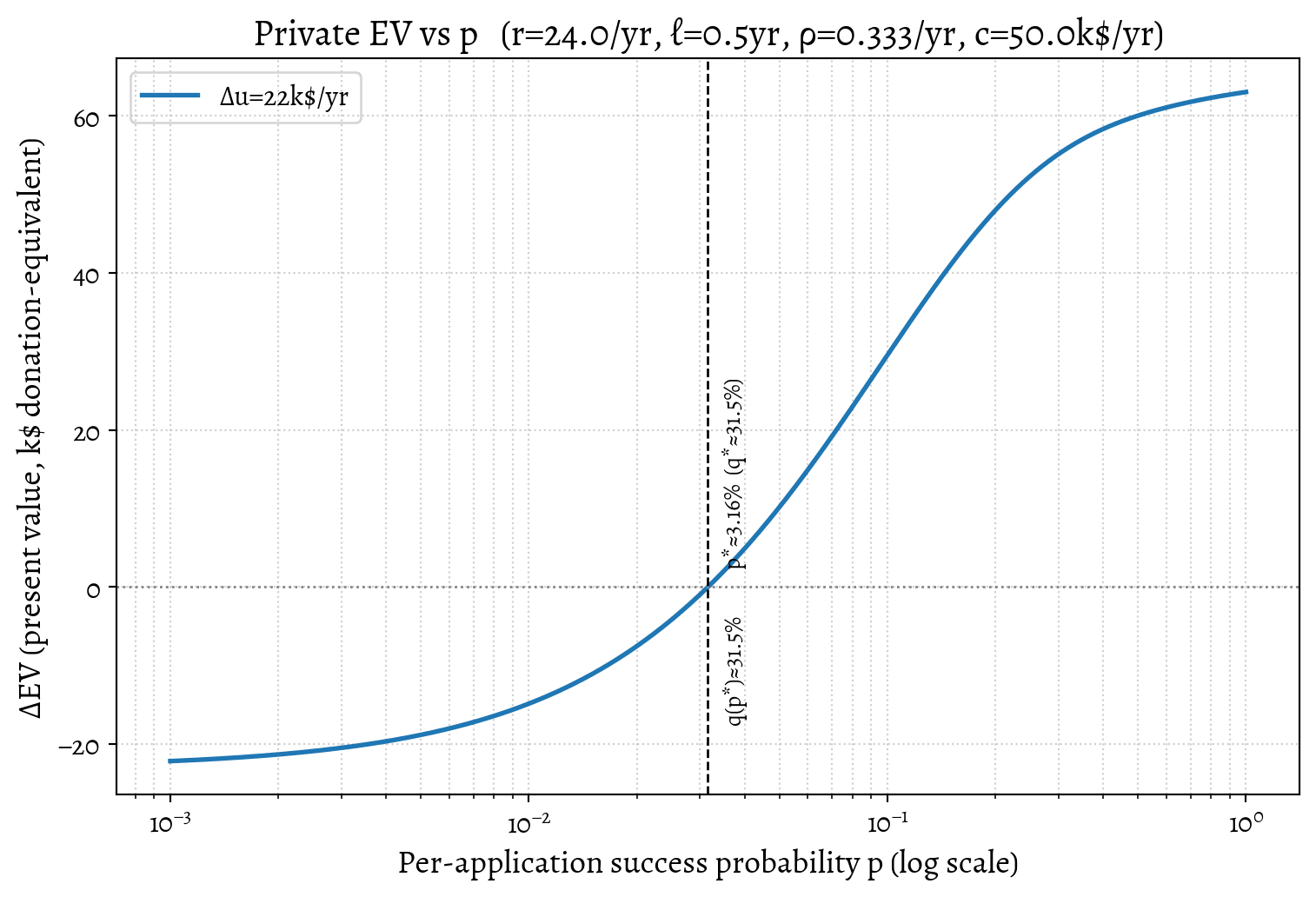
Now, let's plug in some plausible representative numbers for Alice, our mid‑career technical researcher considering a pivot into an AI safety role in a developed economy. She is a successful software engineer taking home $w_0=180$k$/year, donating $d_0=18$k$/year post tax, and having no on-the-job impact $$I_0=0$$ (i.e. No net harm, no net good). Alice earns $w_0=180$, donates $d_0=18$, and has baseline impact $I_0=0$. A target role offers $w_1=120$, $d_1=0$, $I_1=100$. Set $\alpha =1$, runway $\ell =0.5$ years, application rate $r=24$/year, discount $\rho =1/3$, burn $c=50$. Then $\Delta u=(120+0+100)-(180+18+0)=22$ and $$p^{\ast }=\frac{c\rho }{r\Delta u}=\frac{50\cdot \left(1/3\right)}{24\cdot 22}\approx 3.16\%.$$ Over 6 months, the chance of at least one success at $p^{\ast }$ is $q^{\ast }=1-e^{-r{p}^{\ast }\ell }\approx 31.5\%$. Her expected actual sabbatical length is $E\left[\tau \right]=\frac{1-e^{-r{p}^{\ast }\ell }}{r{p}^{\ast }}\approx 0.416\text{years (≈5.0 months)}$, and conditional on success, $E[\tau \mid \text{success}]\approx 0.234\text{years (≈2.8 months)}$. Under these assumptions sabbatical is expected to break even because the job offers enough upside to compensate for greater-than-even risk of failure.

We plot a few values of Alice's to visualize the trade-offs for different upsides $\Delta u$.

If you wish to play around with the assumptions check out the interactive Pivot EV Calculator (source at danmackinlay/career_pivot_calculator).

For Alice, the threshold probability $p^{\ast }$ marks the point where a pivot breaks even; below that, she burns runway faster than expected value, and if she wants to end up making satisfactory impact, she might consider donating money instead. If a 6‑month pivot fails, Alice burns $c\ell=$25k$ that could have been donated now to AI‑safety orgs, and she would have been better off donating that money directly.

Part B --- Field-level model

tl;dr

In world with heavy-tailed distribution of candidate impact, the field benefits from many attempts because a few "hits" dominate. In light-tailed worlds, the same encouragement becomes destructive. We simply don't know which world we're in.

That was Alice's private decision. Let us now consider the field-level perspective. What if everyone has Alice's decision rule? Does that help the world at large? For this we need to add some heterogeneity in candidate quality.

From personal gambles to field strategy

Our goal is to move beyond Alice's private break-even ($p^{\ast }$) to calculate the field's optimum applicant pool size ($K^{\ast }$). This tells us how many Alices society can afford to have 'roll the dice' before the costs of the failures outweigh the value of the discoveries.

We switch from the private ledger of Part A to a public ledger measured in pure impact dollars.

• Private cost (Part A): $c$ includes the individual's full opportunity cost during the sabbatical (foregone wages, consumption, career progression).
• Public cost (Part B): $\gamma$ captures only the foregone public good during the sabbatical: $\gamma =I_0+d_0+\epsilon$ (baseline impact, donations, and externalities). The private wage hit is sad for the candidate but not for the field.

When an individual fails a pivot, they bear the private cost $c$. The field bears the public cost $\gamma$, which captures the tendency that people who are giving up earning to switch to AI safety are donating less etc.

From a field-level perspective, wages and private consumption are transfers and drop out of the analysis; what matters is the net production of public goods, i.e. all that impact we are notionally delivering by working on AI safety.

For this to be anything but trivial, we have to include some way of capturing heterogeneity in candidate quality, otherwise everyone is identical and only one person should ever apply for any job. The minimally complicated way to do this is to assume that each candidate has a different true impact in the role, drawn i.i.d. from some distribution $F$.

• We fix the number of roles per year at $N=r$ and just consider the per-year scale From Alice's perspective the roles were arriving randomly; but from the field's perspective, each year there are a certain number of are fixed and we want to fill them with the best candidates.
• Each applicant $k\in \{1,\dots ,K\}$ has a true per‑year impact in the role $J^{\left(k\right)}\sim F$, i.i.d. (measured in impact dollars per year).
• Employers perfectly observe $J^{\left(k\right)}$ (a strong assumption) and hire the top $N$ candidates.
• Applicants do not observe their own $J^{\left(k\right)}$.
• From a public-goods perspective, each failed pivot costs the field the foregone public impact during the sabbatical, captured by the social burn rate $\gamma$.
• We switch from a time-discounted flow to a steady-state annual perspective; if we do it in continuous time there is lots of annoying book-keeping around sabbatical durations and so on which obscures the main point, so there is a hidden fudge factor here which I am suppressing to keep the algebra simple.

The intuition here is that candidates can bring different capacities for impact, and the field benefits from having more candidates to choose from. The capacity would depend on the role, and include stuff like mathematical ability, interpersonal skills, grit, prestige, access to funding, or strategic personal connections etc.

Let the field‑side annual impact of the hires be the sum of the impact of the top $N$ candidates (we are assuming the employers picks the best $N$ perfectly), $$S_{N,K}:=J_{\left(K\right)}+J_{(K-1)}+\cdots +J_{(K-N+1)}.$$ We care about $B\left(K\right):=E\left[S_{N,K}\right],$ the expected total impact of these best $N$ candidates, and in particular its marginal value each time we add one extra applicant, $${MV}_K:=B(K+1)-B\left(K\right).$$

From a public-good perspective, one failed attempt costs the field $L_{\text{fail},\delta }$ in foregone public impact. Define the social burn rate during sabbatical: $$\gamma :=\$I_0\$+d_0+\epsilon$$ where $$I_0$ $ is the candidate's baseline on-the-job impact per year (often ≈0), $d_0$ is their baseline donations per year, and $\epsilon$ captures any externalities you choose to include (e.g., reviewer time, cohort displacement). Most of a candidate's private consumption loss is a transfer and drops out of the public ledger; what matters socially is the public good that didn't happen during the sabbatical.

The present value of foregone public impact for one failed attempt is: $$L_{\text{fail},\delta }=\gamma {\int }_0^{\ell }{e}^{-\delta t}dt=\gamma \frac{1-e^{-\delta \ell }}{\delta }$$ where $\delta$ is the social discount rate (which we can set equal to $\rho$ for simplicity, though they need not be identical). Under the sabbatical-then-stop rule, all $(K-N)$ unsuccessful candidates impose this cost on the field.

We do not model employer congestion from reviewing lots of applicants --- on the rationale that it is empirically small because employers stop looking at candidates when they're overwhelmed [@Horton2021Jobseekers]. Note, however, that we have also claimed that employers perfectly observe $J^{\left(k\right)}$; which means that we are being optimistic about the field's ability to sort candidates. The social benefit in the model comes from the fact that, all else being equal, more applicants mean a better top‑$N$, and we have more effective researchers doing their research.

1. With $N$ seats fixed, adding one more applicant increases the expected number of failures by exactly 1. Hence the marginal social cost of one extra applicant is $L_{\text{fail},\delta }$, the expected foregone public impact per failed candidate.

2. Whether adding one applicant is socially worthwhile depends on ${MV}_K$.

How much better does one extra applicant make the top-$N$? Extreme value theory tells us this depends on the tail of the candidate quality distribution, $F$ The shape of the tail determines how quickly the marginal value ${MV}_K$ from adding candidates diminishes as the pool $K$ grows.

Tail distributions and diminishing returns

We consider two families: light-tailed (Exponential) and heavy-tailed (Fréchet). Heavy tails capture the intuition that "unicorn" candidates (e.g., 10x engineers) exist and might be waiting in the career-pivot recruiting pool. The exponential family is a light-tailed distribution that decays quickly, and is also super easy to work with, so I've kept it in to check my working on the heavy-tailed case, which is not at all easy to work with.

Light tails: If $J\sim \text{Exp}\left(\lambda \right)$, the marginal value decays hyperbolically: $$MV\_K=\frac{N}{\lambda }\cdot \frac{1}{K+1}.$$ The intuition is that returns diminish quickly; applicants are relatively similar.

Heavy tails: If $J\sim \text{Fréchet}(\alpha ,s)$ (where lower $\alpha$ means heavier tail), the marginal value decays much slower (power law): $$MV\_K\approx C\cdot K^{\frac{1}{\alpha }-1}\text{(for large}K\text{)}.$$ If $\alpha$ is close to 1 (very heavy tail), ${MV}_K$ decays extremely slowly, justifying a wide search for unicorns. As $\alpha$ increases, we recover the light-tailed $1/K$ behaviour.

Field-level optima

Once there are enough people for roles (when $N>K$), adding more applicants ("widening the recruiting funnel") improves the hired cohort on average, because some of the new entrants might be stronger. At the same time, each candidate burning sabbatical time is one more failed attempt that burns public-good resources. We compare these in present-value impact dollars, using a social discount rate $\delta$ (which we can set equal to $\rho$ from Part A for simplicity, though they need not be identical). This rate reflects both time preference and any expected shortening of future impact streams (e.g. job changes, role turnover, project endings).

A filled role produces a stream of impact over time which we will discount, even though we are filling the roles in annualized buckets. The total present value of $$1K$/year of annual impact is \(1K/\delta\) for discount rate \(\delta\).

$$H_{\delta }={\int }_0^{\infty }{e}^{-\delta t}dt=\frac{1}{\delta }\text{(PV weight of one unit of per-year impact).}$$

The total welfare curve $$W\left(K\right)=B\left(K\right)\cdot H_{\delta }-(K-N{)}^{+}\cdot L_{\text{fail},\delta }$$ rises up to a maximum and then declines.

The break-even condition $${MV}_K\cdot H_{\delta }=L_{\text{fail},\delta }$$ therefore defines the welfare-maximizing pool size $K^{\ast }$. $K^{\ast }$ coincides (up to discretization) with the point where the gradient of $W$ changes sign.

Substituting $L_{\text{fail},\delta }=\gamma \frac{1-e^{-\delta \ell }}{\delta }$ and canceling $H_{\delta }=1/\delta$ from both sides gives: $${MV}_K=\gamma (1-e^{-\delta \ell }).$$

The $1/\delta$ factors cancel, so the threshold depends mainly on $\gamma$ and $\ell$ (via the factor $1-e^{-\delta \ell }$).

Solving for the welfare-maximizing pool size $K^{\ast }$ gives:

• Exponential ($J\sim Exp\left(\lambda \right)$, mean $1/\lambda$ in impact dollars): $$K^{\ast }=\frac{N}{\lambda \gamma (1-e^{-\delta \ell })}-1.$$

• Fréchet ($\alpha >1$, scale $s$; $C_N={\sum }_{k=1}^N\Gamma (k-\frac{1}{\alpha })/\Gamma \left(k\right)$): with ${MV}_K\approx \frac{s{C}_N}{\alpha }{K}^{\frac{1}{\alpha }-1}$, $$K^{\ast }={\left(\frac{s{C}_N}{\alpha \gamma (1-e^{-\delta \ell })}\right)}^{\frac{\alpha }{\alpha -1}}.$$ Here $s$ is the Fréchet scale parameter (units of impact per year).

With light tails, there's a finite pool size after which turning up the hype (growing $K$) destroys net welfare. Every extra applicant burns $L_{\text{fail},\delta }$ in foregone public impact while adding ${MV}_K$ that shrinks like $1/K$.

With heavy tails, it's different: As $\alpha \downarrow 1$ increases, $K^{\ast }$ explodes: in very heavy tails, very wide funnels can still be net positive. We might want, as a society, to widen the recruiting funnel relative to the light-tailed case, even if the average candidate quality is the same; it is worth spending a lot of money to find the unicorns.

$$W\left(K\right)=B\left(K\right)\cdot H_{\delta }-max\{K-N,0\}\cdot L_{\text{fail},\delta }$$ Here $B\left(K\right)=E\left[S_{N,K}\right]$ is in impact dollars/year, $H_{\delta }=1/\delta$ converts annual impact to present value, and $L_{\text{fail},\delta }$ is in impact dollars (PV).

• Exponential:

  • $1/\lambda ={\mu }_{\text{imp}}\Rightarrow \lambda =1/{\mu }_{\text{imp}}$.
  • $B\left(K\right)=\frac{N}{\lambda }(1+H_K-H_N)$.

• Fréchet ($\alpha >1$):

  • $E\left[J\right]=s\Gamma (1-1/\alpha )={\mu }_{\text{imp}}\Rightarrow s={\mu }_{\text{imp}}/\Gamma (1-1/\alpha )$.
  • There is not exact form for $B$ but the large-$K$ asymptotic $B\left(K\right)\approx s{C}_N{K}^{1/\alpha }$ with $C_N={\sum }_{k=1}^N\frac{\Gamma (k-\frac{1}{\alpha })}{\Gamma \left(k\right)}$.

We set the expected impact per hire per year to ${\mu }_{\text{imp}}=100$ (impact dollars/yr) to match expected impact Alice's hypothetical target role, but this is just for exposition; you can change it.

We can, of course, plot this.

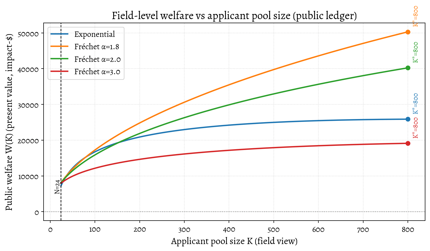
• This plots total net welfare $W\left(K\right)$ and marks the maximum $K^{\ast }$ for each family, showing where total welfare peaks. The dashed line at $K=N$ shows where failures begin: $(K>N\Rightarrow K-N$ people each impose public cost $L_{\text{fail},\delta })$. The markers show $K^{\ast }=\arg maxW\left(K\right)$, the pool size where widening further would reduce total impact.
• Units: $B\left(K\right)$ is in impact dollars per year and is converted to PV by multiplying by $H_{\delta }=\frac{1}{\delta }$. The subtraction uses the discounted per-failure cost $L_{\text{fail},\delta }=\gamma \frac{1-e^{-\delta \ell }}{\delta }$.
• Fréchet curves use the large-$K$ asymptotic $B\left(K\right)\approx s{K}^{1/\alpha }{C}_N$ (with $s={\mu }_{\text{imp}}/\Gamma (1-1/\alpha )$). We could work harder to get exact $B\left(K\right)$ for Fréchet, but the asymptotic is good enough to illustrate the qualitative behaviour.
• We treat all future uncertainties about role duration, turnover, or project lifespan as already captured in the overall discount rate $\delta$.

We can combine these perspectives to visualize the tension between private incentives and public welfare.

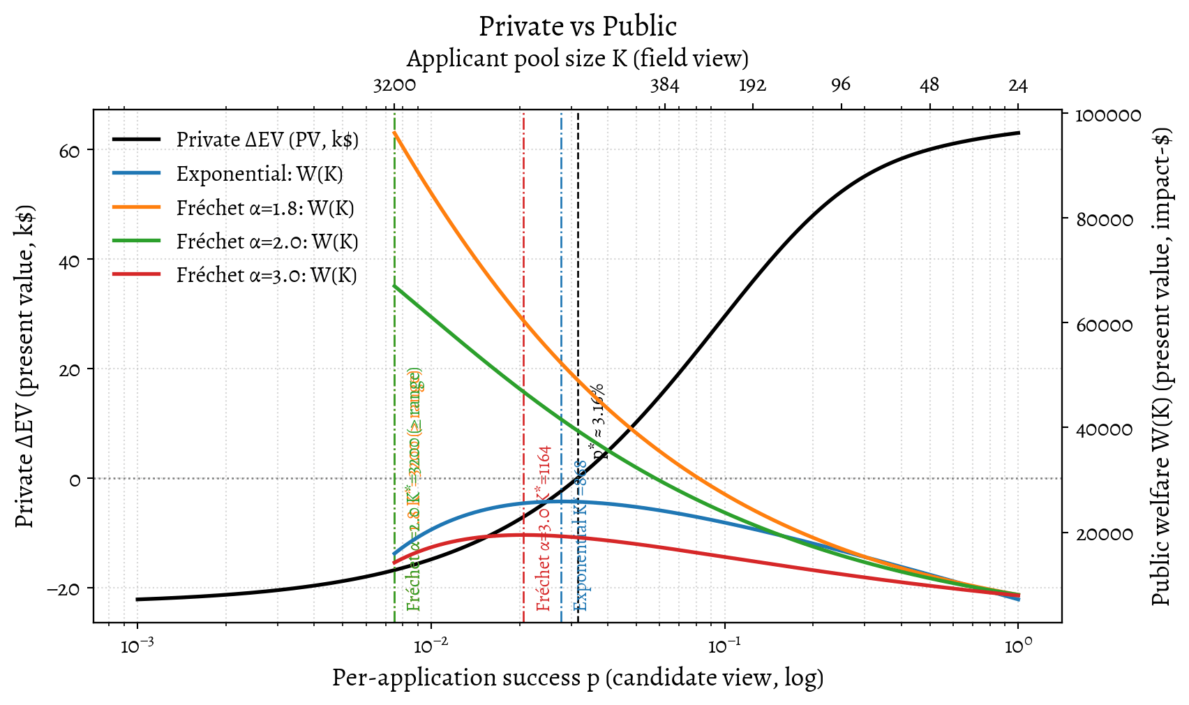
This visualization combines the private and public views by assuming an illustrative mapping between pool size and success probability: $p\approx \beta N/K$ (where $\beta$ bundles screening efficiency; here $\beta =1$). The black curve (left axis) shows the candidate's private EV vs success probability $p$. The colored curves (right axis) show field welfare $W\left(K\right)$. The private break-even $p^{\ast }$ (black dashed line) can fall far to the left of the field-optimal $p\left(K^{\ast }\right)$ (colored vertical lines) This gap represents the region where individuals may be rationally (at a field-level) incentivized to enter, even though the field is already saturated or oversaturated (at a candidate level).

None

Without evidence of heavy tails at your current applicant pool $K$, widening the funnel likely increases social loss.

Part C --- Counterfactual Impact and Equilibrium

Part A modeled a "naive" applicant who evaluates their pivot based on the absolute impact ($I_1$) of the role, ignoring pool dynamics. Part B analyzed the field-level optimum ($K^{\ast }$), showing how the marginal value (${MV}_K$) of an applicant decreases as the pool grows.

Now we tie those together. If Alice is sophisticated, and understands these dynamics and aims to maximize her counterfactual impact, will she make the same choice?

This changes the game, introducing a feedback loop where individual incentives depend on the crowd size ($K$), and the candidate quality distribution $\left(F\right)$.

The Counterfactual Impact Model

If we assume applicants cannot know their quality relative to the pool ex-ante (formally: they are exchangeable), the expected counterfactual impact of the decision to apply is exactly ${MV}_K$ per year.

Alice should use this in her EV calculation. However, the private EV formula (Part A) requires the impact conditional on success, not the ex-ante expected impact due to her decision in isolation.

Let $I_{CF}$ be the expected counterfactual impact conditional on success. Let $q_K$ be the probability of success given the pool size $K$. (In the static model of Part B, with $K+1$ applicants competing for $N$ slots, $q_K=N/(K+1)$). If the attempt fails, the counterfactual impact is zero.

We can derive the relationship (see Appendix): $${MV}_K=q_K\cdot I_{CF}.$$ Therefore, the impact conditional on success is: $$I_{CF}=\frac{{MV}_K}{q_K}.$$ We recalibrate the private decision by defining the counterfactual private surplus, $\Delta u_{CF}$, replacing the naive absolute impact $I_1$ with the counterfactual estimate $I_{CF}$.

This changes the dynamics; previously the gamble's even depended on the pool size only insofar as it affected the per-application success probability $p$ and thus the overall success probability $q_K$. Now the value of the upside also depends on the pool size $K$. As $K$ grows, ${MV}_K$ decreases, but $q_K$ also decreases. The behavior of $I_{CF}$ depends on how these balance, which is determined by the tail of the impact distribution.

The Dynamics of Counterfactual Impact

The behavior of $I_{CF}$ leads to different implications depending on whether the recruitment pool is light-tailed or heavy-tailed.

Case 1: Light Tails

In a light-tailed recruitment pool (where applicants are relatively similar), the math reveals (See Appendix) that the expected counterfactual impact conditional on success, $I_{CF}$, is constant and equal to the population average impact ($\mu$), regardless of how crowded the field is ($K$). $$I_{CF}=\mu \text{(Light Tail)}$$ Intuition: While a larger pool increases the quality of the very best hire, it also increases the quality of the person they displace. In the stylized light-tailed model (Exponential distribution), these effects perfectly cancel out. More generally, in light-tailed talent pools, the gap between the hire and the displaced candidate does not grow significantly with the pool size.

Implication: If the average impact $\mu$ is modest and the candidate skills are relatively evenly distributed, pivots involving significant pay cuts are likely negative EV for the average applicant, no matter the pool size.

Case 2: Heavy Tails

In a heavy-tailed model, "unicorns" are hiding in the recruiting pool. Here, $I_{CF}$ increases as the field gets more crowded ($K$), and undert certain assumptions can increase fast enough to offset the costs of all the sabbaticals and foregone donations etc. For Fréchet with shape $\alpha$, $I_{CF}$ grows proportionally to $K^{1/\alpha }$. $$I_{CF}\propto K^{1/\alpha }\text{(Heavy Tail)}$$ Intuition: As $K$ increases, the expected quality of the top candidates increases significantly faster than the quality of the candidates they displace. Success in a large pool is a strong signal that you are likely a high-impact individual, and the gap between you and the displaced candidate is large.

Implication: In a heavy-tailed world, the pivot can become highly attractive if the field is sufficiently crowded, even with significant pay cuts.

Alice Revisited

Alice revisited. With light‑tailed assumptions, $I_{CF}$ equals the population mean $\mu$ and is too small to offset Alice's pay cut and lost donations---her counterfactual surplus is negative regardless of $K$. Under heavy‑tailed assumptions, $I_{CF}$ rises with $K$; under a broad range of conditions, the pivot can become attractive despite large pay cuts (i.e. if Alice truly might be a unicorn). The sign and size of this effect hinge on the tail parameter and scale, which are currently unmeasured.

Visualizing Private Incentives vs. Public Welfare

We can now visualize the dynamics of private, public and counterfactual private valuations together by assuming an illustrative mapping between pool size and success probability: $p\approx \beta N/K$. This allows us to see how the incentives change as the field gets more crowded (moving left on the x-axis).

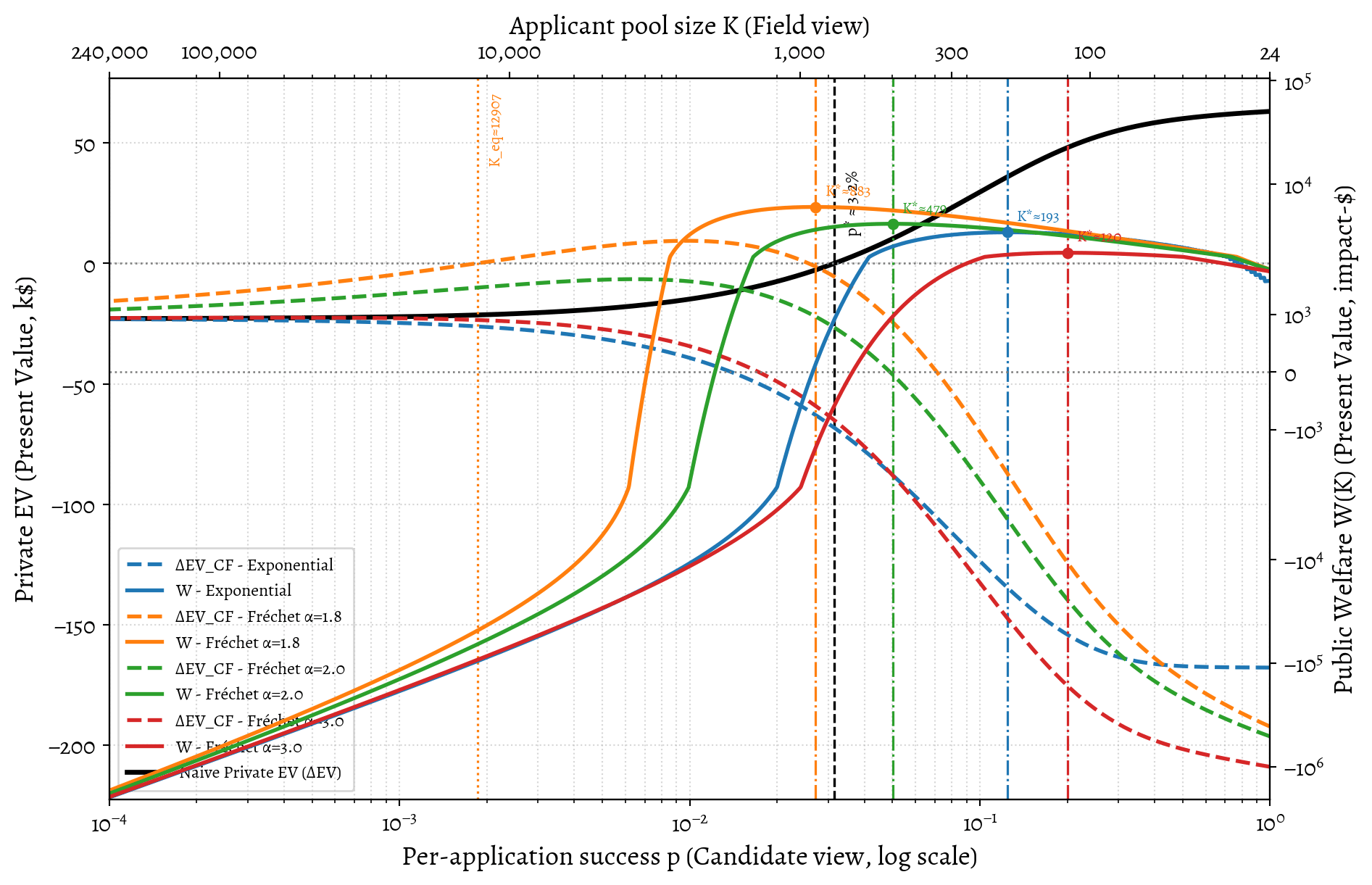
This visualization combines all three perspectives using Alice's parameters. There are a lot of lines and a lot of assumptions wrapped up in this one plot. The main takeaway is that if you care about solving the problem, for many variants of this model, in a trade-off of pivoting versus donating, you should probably donate. The only exception is if you believe the talent pool is very heavy-tailed (Fréchet with $\alpha \le 2$); in which case if you are one of those unicorns you should probably pivot. Otherwise, donating is likely to have higher expected impact.

• Left Axis (Private EV):

  • A (Black Solid): The naive applicant's EV (Part A). Crosses zero at the naive break-even $p^{\ast }\approx 3.16\%$.
  • C (Colored Dashed): The sophisticated applicant's EV (Part C), using counterfactual impact $\Delta u_{CF}\left(K\right)$. Where these curves cross zero defines the equilibrium $K_{eq}$.

• Right Axis (Public Welfare):

  • B (Colored Solid): The field's total welfare $W\left(K\right)$ (Part B). The peak defines the social optimum $K^{\ast }$.

1. The Information Gap (A vs C): 1. The Information Gap (A vs C): The Naive EV (Black) is significantly higher than the Counterfactual EV (Colored Dashed) across most of the range. Applicants relying on naive valuations of the impact of a career pivot (using personal impact change $\Delta I$ rather than rather than counterfactual impact change $\Delta I_{CF}$) will drastically overestimate their counterfactual impact, and thus the expected value of the pivot.

2. The Impact of Costs vs. Tails:

   • In light-tailed talent pools (Exponential, Purple; Fréchet $\alpha =3.0$, Red), the Counterfactual EV is always negative. Alice's 78k financial loss dominates the expected impact. The equilibrium is minimal ($K_{eq}=N$), leading to Under-Entry relative to the optimum ($K^{\ast }$).
   • In heavy-tailed talent pools (Fréchet $\alpha =2.0$, Green; $\alpha =1.8$, Orange), the dynamics change dramatically.

3. Complex Dynamics in Heavy Tails (The "Hump Shape"): For heavy tails (Green, Orange dashed lines), the Counterfactual EV is non-monotonic. It starts positive, increases as $K$ grows (because $I_{CF}\left(K\right)$ increases rapidly), and eventually decreases as the success probability $p\left(K\right)$ drops too low.

4. The Structural Misalignment (B vs C): In heavy-tailed talent pools, the equilibrium $K_{eq}$ is vastly larger than the optimum $K^{\ast }$. The efficient search process (high $r$) means the private cost of trying is low, incentivizing entry long past the social optimum. This leads to massive over-entry. (For example, in the $\alpha =2.0$ case, $K^{\ast }$ is around 30k, while $K_{eq}$ is over 400k).

This visualization confirms the analysis: the system's calibration is highly sensitive to the tail distribution and private costs. Depending on the parameters, the system can structurally incentivize either severe under-entry or massive over-entry, even if applicants are sophisticated.

Equilibrium vs. Optimum

This feedback mechanism---where incentives depend on $K$---creates a natural equilibrium. Applicants will enter until the EV for the marginal entrant is zero. This defines the equilibrium candidate pool size, $K_{eq}$.

To analyze this, we must reintegrate the counterfactual surplus $\Delta u_{CF}\left(K\right)$ into the dynamic search model (Part A). We assume the pool size $K$ determines the surplus $\Delta u_{CF}\left(K\right)$ and the per-application success probability $p\left(K\right)$. The equilibrium $K_{eq}$ occurs when the expected gain rate equals the burn rate (the bracketed term in the EV formula is zero): $$\frac{\Delta u_{CF}\left(K\right)rp\left(K\right)}{\rho }=c.$$ Does this equilibrium $K_{eq}$ align with the socially optimal pool size $K^{\ast }$ (Part B)?

Generally, no. The alignment depends on the comparison between private costs ($c$), social costs ($\gamma$), and the efficiency of the job search process ($r$).

Search Efficiency

The equilibrium condition reveals a dependence on the application rate $r$. We can rewrite the equilibrium condition as: $$\Delta u_{CF}\left(K\right)\cdot p\left(K\right)=\frac{c\rho }{r}.$$ The left side is the expected counterfactual surplus per application attempt. The right side, $\frac{c\rho }{r}$, represents the effective private cost hurdle per application attempt (scaled by the discount rate).

If the job search process is highly efficient (high $r$), the private cost hurdle is low. This encourages individuals to enter even when the expected counterfactual impact per application is small, because trying is cheap.

We can compare this private incentive to the social optimum. As derived in Appendix C.3, if the private cost hurdle ($\frac{c\rho }{r}$) is significantly lower than the social cost of failure (related to $\gamma$), the system structurally leads to Over-Entry ($K_{eq}>K^{\ast }$).

Let's check Alice's numbers: $c=50,\rho =1/3,r=24$. The private cost hurdle is $\frac{c\rho }{r}\approx \frac{50/3}{24}\approx 0.69k$. The social cost rate $\gamma$ (foregone donations) is $18k$.

Since $0.69k\ll 18k$, the system strongly favors over-entry. The efficiency of the search process dramatically lowers the private barrier to entry compared to the social costs incurred.

For example, in the heavy-tailed case ($\alpha =2$), we might find $K^{\ast }\approx 11,600$, while $K_{eq}\approx 178,000$.

Implications and Solutions

The analysis suggests the AI safety field may be oversubscribed. The core problem is misalignment: organizations influencing the funnel size do not internalize the costs borne by unsuccessful applicants. This incentivizes maximizing application volume (a visible proxy) rather than welfare-maximizing matches---a classic setup for Goodhart's Law.

A healthy field can rationally accept high individual failure rates if it measures and communicates the odds. An unmeasured one turns the same logic into waste. The ethical burden shifts when the system knowingly asks people to take low-probability gambles without making that explicit.

For Individuals: Knowing the Game

For mid-career individuals, the decision is high-stakes. (For early-career individuals, costs $c$ are lower, making the gamble more favorable, but the need to estimate $p$ remains.)

1. Calculate your threshold ($p^{\ast }$): Use the model in Part A (and the linked calculator). Without strong evidence that $p>p^{\ast }$, a pivot involving significant unpaid time is likely EV-negative.
2. Seek cheap signals: Seek personalized evidence of fit---such as applying to a few roles before leaving your current job---before committing significant resources.
3. Use grants as signals: Organizations like Open Philanthropy offer career transition grants. These serve as information gates. If received, a grant lowers the private cost ($c$). If denied, it is a valuable calibration signal. If a major funder declines to underwrite the transition, candidates should update $p$ downwards. (If you don't get that Open Phil transition grant, don't quit your current job.)

For Organizations: Transparency and Feedback

Employers and advice organizations control the information flow. Until they provide evidence-based estimates of success probabilities, their generic encouragement should be treated with skepticism.

1. Publish stage-wise acceptance rates (Base Rates). Employers must publish historical data (applicants, interviews, offers) by track and seniority. This is the single most impactful intervention for anchoring $p$.
2. Provide informative feedback and rank. Employers should provide standardized feedback or an indication of relative rank (e.g., "top quartile"). This feedback is costly, but this cost must be weighed against the significant systemic waste currently externalized onto applicants and the long-term credibility of the field.
3. Track advice calibration. Advice organizations should track and publish their forecast calibration (e.g., Brier scores) regarding candidate success. If an advice organization does not track outcomes, its advice cannot be calibrated except by coincidence.

For the Field: Systemic Calibration

To optimize the funnel size, the field needs to measure costs and impact tails.

1. Estimate applicant costs ($c\ell$). Advice organizations or funders should survey applicants (successful and unsuccessful) to estimate typical pivot costs.
2. Track realized impact proxies. Employers should analyze historical cohorts to determine if widening the funnel is still yielding significantly better hires, or if returns are rapidly diminishing.
3. Experiment with mechanism design. In capacity-constrained rounds, implementing soft caps---pausing applications after a certain number---can reduce applicant-side waste without significantly harming match quality [@Horton2024Reducing].

Where next?

I'd like feedback from people deeper in the AI safety career ecosystem. I'd love to chat with people from 80,000 Hours, MATS, FHI, CHAI, Redwood Research, Anthropic, etc., about this. What is your model about the candidate impact distribution, the tail behaviour, and the costs? What have I got wrong? What have I missed? I'm open to the possibility that this is well understood and being actively managed behind the scenes, but I haven't seen it laid out this way anywhere.

Further reading

Resources that complement the mechanism-design view of the AI safety career ecosystem:

• Christopher Clay, AI Safety's Talent Pipeline is Over-optimised for Researchers
• AI Safety Field Growth Analysis 2025
• Why experienced professionals fail to land high-impact roles Context deficits and transition traps that explain why even strong senior hires often bounce out of the AI safety funnel.
• Levelling Up in AI Safety Research Engineering --- EA Forum. A practical upskilling roadmap; complements the "lower $c$, raise $V$, raise $p$" levers by reducing risk before a pivot.
• SPAR AI --- Safety Policy and Alignment Research program. An example of a program that provides structured training and, implicitly, some "negative previews" of the grind of AI safety work.
• MATS retrospectives --- LessWrong. Transparency on acceptance rates, alumni experiences, and obstacles faced in this training program.
• Why not just send people to Bluedot on FieldBuilding Substack. A critique of naive funnel-building and the hidden costs of over-sending candidates to "default" programs.
• How Stuart Russell's IASEAI conference failed to live up to its potential (FBB #8) --- EA Forum. A cautionary tale about how even well-intentioned field-building efforts can misfire without mechanism design.
• 80,000 Hours career change guides. Practical content on managing costs, transition grants, and opportunity cost---useful for calibrating $c$ in the pivot-EV model.
• Forecasting in personal decisions --- 80k. Advice on making and updating stage-wise probability forecasts; relevant to candidate calibration.
• AI safety technical research - Career review
• Updates to our research about AI risk and careers - 80,000 Hours
• The case for taking your technical expertise to the field of AI policy - 80,000 Hours
• Center for the Alignment of AI Alignment Centers. A painfully relatable satire that needs citing here.

Appendix: Mathematical Details

Part A: Private Decision Model Derivations

We model the career pivot attempt as a continuous-time process during a sabbatical of maximum length $\ell$.

Setup:

• Job opportunities arrive as a Poisson process with rate $r$.
• Per-application success probability is $p$ (i.i.d.).
• The success process is a Poisson process with rate $\lambda =rp$.
• The time to the first success is $T_1\sim Exp\left(\lambda \right)$.
• The actual sabbatical duration is the stopping time $\tau =min\{T_1,\ell \}$.
• The continuous discount rate is $\rho >0$.
• The annual utility surplus if the pivot succeeds is $\Delta u$.
• The burn rate during the sabbatical is $c$.

Sabbatical Duration and Success Statistics

The probability of success within the runway is: $$q=P(T_1\le \ell )=1-e^{-\lambda \ell }=1-e^{-rp\ell }.$$ We calculate the expected duration $E\left[\tau \right]$ using the survival function $P(\tau >t)$. For $t\in [0,\ell ]$, $\tau >t$ if and only if no success has occurred by time $t$, so $P(\tau >t)=P(T_1>t)=e^{-\lambda t}$. $P(\tau >t)=0$ for $t>\ell$. $$E\left[\tau \right]={\int }_0^{\infty }P(\tau >t)dt={\int }_0^{\ell }{e}^{-\lambda t}dt=\frac{1-e^{-\lambda \ell }}{\lambda }.$$ The expected duration conditional on success, $E[\tau \mid \text{success}]=E[T_1\mid T_1\le \ell ]$, uses the truncated exponential distribution. The PDF of $T_1$ conditional on $T_1\le \ell$ is $f(t\mid T_1\le \ell )=\frac{\lambda e^{-\lambda t}}{1-e^{-\lambda \ell }}$ for $t\in [0,\ell ]$. Using integration by parts: $$\begin{array}{ccccc}E[\tau \mid \text{success}]& =\frac{1}{1-e^{-\lambda \ell }}{\int }_0^{\ell }t\lambda e^{-\lambda t}dt& =\frac{1}{1-e^{-\lambda \ell }}({[-t{e}^{-\lambda t}]}_0^{\ell }+{\int }_0^{\ell }{e}^{-\lambda t}dt)& =\frac{1}{1-e^{-\lambda \ell }}(-\ell e^{-\lambda \ell }+\frac{1-e^{-\lambda \ell }}{\lambda })& =\frac{1}{\lambda }-\frac{\ell e^{-\lambda \ell }}{1-e^{-\lambda \ell }}.\end{array}$$

Derivation of the Expected Present Value ($\Delta {EV}_{\rho }\left(p\right)$)

The expected value of the pivot attempt is the expected discounted benefit minus the expected discounted cost.

Expected Discounted Benefit ($E\left[B\right]$): If success occurs at time $T_1=t\le \ell$, the benefit is the present value (PV) of the stream $\Delta u$ starting at $t$: $B\left(t\right)={\int }_t^{\infty }\Delta u{e}^{-\rho (s-t)}{e}^{-\rho t}ds=\frac{\Delta u}{\rho }{e}^{-\rho t}$. The expectation is taken over the time of success $T_1$, up to the runway limit $\ell$, using the density $f_{T_1}\left(t\right)=\lambda e^{-\lambda t}$: $$\begin{array}{cccc}E\left[B\right]& ={\int }_0^{\ell }B\left(t\right)f_{T_1}\left(t\right)dt={\int }_0^{\ell }\frac{\Delta u}{\rho }{e}^{-\rho t}\lambda e^{-\lambda t}dt& =\frac{\Delta u\lambda }{\rho }{\int }_0^{\ell }{e}^{-(\lambda +\rho )t}dt& =\frac{\Delta u\lambda }{\rho (\lambda +\rho )}(1-e^{-(\lambda +\rho )\ell }).\end{array}$$

Expected Discounted Cost ($E\left[C\right]$): The cost is incurred at rate $c$ during the sabbatical $[0,\tau ]$. We calculate $E\left[{\int }_0^{\tau }c{e}^{-\rho t}dt\right]$. We swap expectation and integration (by Fubini's theorem, as the integrand is positive): $$E\left[C\right]=c{\int }_0^{\infty }{e}^{-\rho t}E\left[I\right(t<\tau \left)\right]dt=c{\int }_0^{\infty }{e}^{-\rho t}P(\tau >t)dt.$$ Using the survival function $P(\tau >t)=e^{-\lambda t}$ for $t\in [0,\ell ]$: $$E\left[C\right]=c{\int }_0^{\ell }{e}^{-\rho t}{e}^{-\lambda t}dt=c{\int }_0^{\ell }{e}^{-(\lambda +\rho )t}dt=c\frac{1-e^{-(\lambda +\rho )\ell }}{\lambda +\rho }.$$

Total Expected Value: $$\Delta {EV}_{\rho }\left(p\right)=E\left[B\right]-E\left[C\right].$$ Factoring out the common term $\frac{1-e^{-(\lambda +\rho )\ell }}{\lambda +\rho }$ (the expected discounted duration) and substituting $\lambda =rp$: $$\Delta {EV}_{\rho }\left(p\right)=\frac{1-e^{-(rp+\rho )\ell }}{rp+\rho }(\frac{\Delta urp}{\rho }-c).$$

Break-even Probability ($p^{\ast }$)

The EV is zero when the bracketed term is zero (since the prefactor is strictly positive). $$\frac{\Delta ur{p}_{\rho }^{\ast }}{\rho }-c=0⟹p_{\rho }^{\ast }=\frac{c\rho }{r\Delta u}.$$

Part B: Field-Level Model Derivations

We analyze the field-level optimum using a public ledger in impact dollars.

Setup:

• $K$ applicants, $N$ seats. Impacts $J^{\left(k\right)}\sim F$ i.i.d.
• Hires are the top $N$ order statistics: $J_{\left(K\right)}\ge J_{(K-1)}\ge \dots$.
• Expected annual benefit $B\left(K\right)=E\left[{\sum }_{k=K-N+1}^K{J}_{\left(k\right)}\right]$.
• Marginal value ${MV}_K=B(K+1)-B\left(K\right)$.
• Social discount rate $\delta$.
• Social burn rate (foregone public impact) $\gamma$.

We do not model congestion costs. Generally, employers who have filled a given role can just ignore excess applications, and there's a lot of evidence to suggest that they do so [@Horton2017Digital; @Horton2021Jobseekers; @Horton2024Reducing].

Welfare Function and Optimality

Present Value Horizon: $H_{\delta }={\int }_0^{\infty }{e}^{-\delta t}dt=1/\delta$.

PV of Failed Attempt: Assuming a failed attempt uses the full runway $\ell$ (this simplifies the calculation of the marginal cost of an additional applicant): $$L_{\text{fail},\delta }={\int }_0^{\ell }\gamma e^{-\delta t}dt=\gamma \frac{1-e^{-\delta \ell }}{\delta }.$$

Total Welfare ($W\left(K\right)$): $$W\left(K\right)=B\left(K\right)\cdot H_{\delta }-max\{K-N,0\}\cdot L_{\text{fail},\delta }.$$ The welfare-maximizing pool size $K^{\ast }$ occurs (for $K>N$) when the marginal benefit equals the marginal cost. Adding one applicant adds exactly one expected failure, so the marginal cost is $L_{\text{fail},\delta }$. $${MV}_K\cdot H_{\delta }=L_{\text{fail},\delta }.$$ Substituting the expressions and canceling $1/\delta$: $${MV}_K=\gamma (1-e^{-\delta \ell }).$$

Distribution-Specific Results

We solve for $K^{\ast }$ based on the behavior of ${MV}_K$ for different distributions $F$.

Exponential Distribution (Light Tail)

Let $J\sim Exp\left(\lambda \right)$, with mean $1/\lambda$. The expected sum of the top $N$ order statistics out of $K$ draws has a known closed form, often derived using the Rényi representation of exponential spacings: $$B\left(K\right)=\frac{N}{\lambda }(1+H_K-H_N),$$ where $H_K={\sum }_{k=1}^K\frac{1}{k}$ is the $K$-th harmonic number.

Marginal Value: $${MV}_K=B(K+1)-B\left(K\right)=\frac{N}{\lambda }(H_{K+1}-H_K)=\frac{N}{\lambda (K+1)}.$$ Returns diminish hyperbolically ($O\left(1/K\right)$).

Optimal Pool Size $K^{\ast }$: Setting ${MV}_K$ equal to the marginal social cost $\gamma (1-e^{-\delta \ell })$: $$K^{\ast }=\frac{N}{\lambda \gamma (1-e^{-\delta \ell })}-1.$$

Fréchet Distribution (Heavy Tail)

Let $J\sim \text{Fréchet}(\alpha ,s)$, with shape $\alpha >1$ (required for finite mean) and scale $s$. We use asymptotic results from Extreme Value Theory for large $K$. The expected sum of the top $N$ scales as $K^{1/\alpha }$: $$B\left(K\right)\approx s{K}^{1/\alpha }{C}_N\left(\alpha \right),$$ where $C_N\left(\alpha \right)$ is a constant independent of $K$ and $s$: $$C_N\left(\alpha \right):=\sum _{k=1}^N\frac{\Gamma (k-\frac{1}{\alpha })}{\Gamma \left(k\right)}.$$

Marginal Value: We approximate the marginal value using the derivative of the asymptotic expression: $${MV}_K\approx \frac{d}{dK}B\left(K\right)=s{C}_N\left(\alpha \right)\frac{1}{\alpha }{K}^{\frac{1}{\alpha }-1}.$$ Returns diminish as a power law ($O\left(K^{-(1-1/\alpha )}\right)$), slower than Exponential.

Optimal Pool Size $K^{\ast }$: Setting ${MV}_K$ equal to the marginal social cost $\gamma (1-e^{-\delta \ell })$ and solving for $K$: $$\frac{s{C}_N\left(\alpha \right)}{\alpha }(K^{\ast }{)}^{\frac{1}{\alpha }-1}=\gamma (1-e^{-\delta \ell }).$$ $$K^{\ast }={\left(\frac{s{C}_N\left(\alpha \right)}{\alpha \gamma (1-e^{-\delta \ell })}\right)}^{\frac{\alpha }{\alpha -1}}.$$ As $\alpha \downarrow 1$ (heavier tails), the exponent $\frac{\alpha }{\alpha -1}\to \infty$, causing $K^{\ast }$ to explode.

Appendix C: Counterfactual Impact and Equilibrium Derivations

Derivation of $I_{CF}$

We want to relate the Marginal Value of entry (${MV}_K$) to the expected counterfactual impact conditional on success ($I_{CF}$).

${MV}_K$ is the expected increase in total field impact when an applicant joins the pool (moving from $K$ to $K+1$ applicants). Let $S$ be the event of success (being hired). $q_K$ is the probability of success $P\left(S\right)$. We assume applicants are exchangeable.

By the law of total expectation: $${MV}_K=E[\text{Impact of Entry}\mid S]P\left(S\right)+E[\text{Impact of Entry}\mid \neg S]P\left(\neg S\right).$$ If the applicant enters and fails ($\neg S$), their counterfactual impact is 0. The expected impact conditional on success is $I_{CF}$.

Therefore: $${MV}_K=I_{CF}\cdot q_K.$$ Assuming exchangeable applicants competing for $N$ slots in a pool of $K+1$, $q_K=N/(K+1)$. $$I_{CF}=\frac{{MV}_K}{q_K}={MV}_K\cdot \frac{K+1}{N}.$$

C.2 $I_{CF}$ for Distributions

Exponential (Light Tail): Mean impact $\mu$. From Appendix B, ${MV}_K=N\mu /(K+1)$. $$I_{CF}=\frac{N\mu /(K+1)}{N/(K+1)}=\mu .$$ The expected counterfactual impact conditional on success is constant.

Fréchet (Heavy Tail): From Appendix B, ${MV}_K\propto K^{1/\alpha -1}$ (asymptotically for large K). $q_K\propto 1/K$. $$I_{CF}=\frac{{MV}_K}{q_K}\propto \frac{K^{1/\alpha -1}}{1/K}=K^{1/\alpha }.$$ The expected counterfactual impact conditional on success grows with the pool size $K$.

C.3 Equilibrium Condition and Misalignment

The equilibrium $K_{eq}$ occurs when the private EV, using the counterfactual surplus $\Delta u_{CF}\left(K\right)$, is zero. This happens when the bracketed term in the EV formula (Part A) is zero: $$\frac{\Delta u_{CF}\left(K\right)rp\left(K\right)}{\rho }-c=0⟹\Delta u_{CF}\left(K\right)\cdot p\left(K\right)=\frac{c\rho }{r}.$$ The RHS, $\frac{c\rho }{r}$, is the effective private cost hurdle per application attempt.

We compare this to the social optimality condition $K^{\ast }$, defined in Part B. For simplicity, we approximate the social cost of failure $L_{\text{fail},\delta }\approx \gamma /\delta$ (assuming large $\ell$) and set $\delta =\rho$. The optimality condition ${MV}_K\cdot H_{\delta }=L_{\text{fail},\delta }$ becomes: $${MV}_K=\gamma .$$

Analyzing Over/Under Entry:

To illustrate the misalignment, consider a simplified case where private financial losses (pay cuts) are negligible, so $\Delta u_{CF}\left(K\right)\approx I_{CF}\left(K\right)$. Also assume the per-application success rate $p\left(K\right)$ approximates the overall success probability $q_K$.

In this case, $\Delta u_{CF}\left(K\right)\cdot p\left(K\right)\approx I_{CF}\left(K\right)\cdot q_K={MV}_K$.

The private equilibrium condition simplifies to: ${MV}_K=\frac{c\rho }{r}$. The social optimum condition remains: ${MV}_K=\gamma$.

Since ${MV}_K$ is decreasing in $K$, $K_{eq}>K^{\ast }$ (Over-Entry) occurs if the private threshold is lower than the social threshold: $$\frac{c\rho }{r}<\gamma .$$ This happens when the private cost hurdle per attempt is less than the social cost rate of failure. As shown in the main text using Alice's parameters (0.69k vs 18k), this inequality often holds strongly, indicating a structural tendency toward over-entry even with sophisticated, counterfactual reasoning.

References

---

1. To be consistent we need to take this to be a local linear approximation at your current wage and impact level; so we are implicitly looking at marginal utility. ↩︎