A recent post by Simon_M argued that StrongMinds should not be a top recommended charity (yet), and many people seemed to agree. While I think Simon raised several useful points regarding StrongMinds, he didn't engage with the cost-effectiveness analysis of StrongMinds that I conducted for the Happier Lives Institute (HLI) in 2021 and justified this decision on the following grounds:
“Whilst I think they have some of the deepest analysis of StrongMinds, I am still confused by some of their methodology, it’s not clear to me what their relationship to StrongMinds is.”.
By failing to discuss HLI’s analysis, Simon’s post presented an incomplete and potentially misleading picture of the evidence base for StrongMinds. In addition, some of the comments seemed to call into question the independence of HLI’s research. I’m publishing this post to clarify the strength of the evidence for StrongMinds, HLI’s independence, and to acknowledge what we’ve learned from this discussion.
I raise concerns with several of Simon’s specific points in a comment on the original post. In the rest of this post, I’ll respond to four general questions raised by Simon’s post that were too long to include in my comment. I briefly summarise the issues below and then discuss them in more detail in the rest of the post
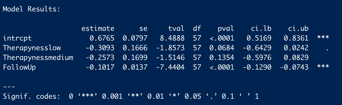
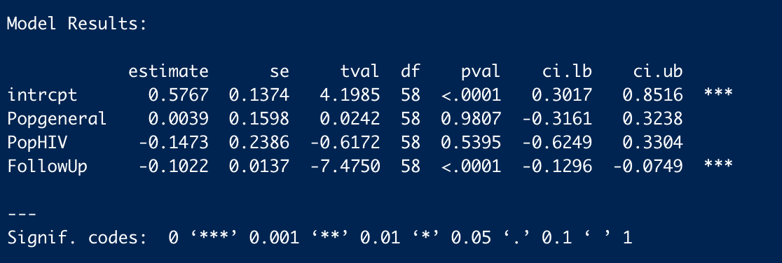
1. Should StrongMinds be a top-rated charity? In my view, yes. Simon claims the conclusion is not warranted because StrongMinds’ specific evidence is weak and implies implausibly large results. I agree these results are overly optimistic, so my analysis doesn’t rely on StrongMind’s evidence alone. Instead, the analysis is based mainly on evidence synthesised from 39 RCTs of primarily group psychotherapy deployed in low-income countries.
2. When should a charity be classed as “top-rated”? I think that a charity could be considered top-rated when there is strong general evidence OR charity-specific evidence that the intervention is more cost-effective than cash transfers. StrongMinds clears this bar, despite the uncertainties in the data.
3. Is HLI an independent research institute? Yes. HLI’s mission is to find the most cost-effective giving opportunities to increase wellbeing. Our research has found that treating depression is very cost-effective, but we’re not committed to it as a matter of principle. Our work has just begun, and we plan to publish reports on lead regulation, pain relief, and immigration reform in the coming months. Our giving recommendations will follow the evidence.
4. What can HLI do better in the future? Communicate better and update our analyses. We didn’t explicitly discuss the implausibility of StrongMinds’ data in our work. Nor did we push StrongMinds to make more reasonable claims when we could have done so. We acknowledge that we could have done better, and we will try to do better in the future. We also plan to revise and update our analysis of StrongMinds before Giving Season 2023.
1. Should StrongMinds be a top-rated charity?
I agree that StrongMinds’ claims of curing 90+% of depression are overly optimistic, and I don’t rely on them in my analysis. This figure mainly comes from StrongMinds’ pre-post data rather than a comparison between a treatment group and a control. These data will overstate the effect because depression scores tend to decline over time due to a natural recovery rate. If you monitored a group of depressed people and provided no treatment, some would recover anyway.
My analysis of StrongMinds is based on a meta-analysis of 39 RCTS of group psychotherapy in low-income countries. I didn’t rely solely on StrongMinds’ own evidence alone, I incorporated the broader evidence base from other similar interventions too. This strikes me, in a Bayesian sense, as the sensible thing to do. In the end, StrongMinds' controlled trials only make up 21% of the effect of the estimate (see Section 4 of the report for a discussion of the evidence base). It's possible to quibble with the appropriate weight of this evidence, but the key point is that it is much less than the 100% Simon seems to suggest.
2. When should a charity be classed as “top-rated”?
At HLI, we think the relevant factors for recommending a charity are:
(1) cost-effectiveness is substantially better than our chosen benchmark (GiveDirectly cash transfers); and
(2) strong evidence of effectiveness.
I think Simon would agree with these factors, but we define “strong evidence” differently.
I think Simon would define “strong evidence” as recent, high-quality, and charity-specific. If that’s the case, I think that’s too stringent. That standard would imply that GiveWell should not recommend bednets, deworming, or vitamin-A supplementation. Like us, GiveWell also relies on meta-analyses of the general evidence (not charity-specific data) to estimate the impact of malaria prevention (AMF, row 36) and vitamin-A supplementation (HKI, row 24) on mortality, and they use historical evidence for the impact of malaria prevention on income (AMF, row 109). Their deworming CEA infamously relies on a single RCT (DtW, row 7) of a programme quite different from the one deployed by the deworming charities they support.
In an ideal world, all charities would have the same quality of evidence that GiveDirectly does (i.e., multiple, high-quality RCTs). In the world we live in, I think GiveWell’s approach is sensible: use high-quality, charity-specific evidence if you have it. Otherwise, look at a broad base of relevant evidence.
As a community, I think that we should put some weight on a recommendation if it fits the two standards I listed above, according to a plausible worldview (i.e., GiveWell’s moral weights or HLI’s subjective wellbeing approach). All that being said, we’re still developing our charity evaluation methodology, and I expect our views to evolve in the future.
3. Is HLI an independent research institute?
In the original post, Simon said:
I’m going to leave aside discussing HLI here. Whilst I think they have some of the deepest analysis of StrongMinds, I am still confused by some of their methodology, it’s not clear to me what their relationship to StrongMinds is (emphasis added).
The implication, which others endorsed in the comments, seems to be that HLI’s analysis is biased because of a perceived relationship with StrongMinds or an entrenched commitment to mental health as a cause area which compromises the integrity of our research. While I don’t assume that Simon thinks we’ve been paid to reach these conclusions, I think the concern is that we’ve already decided what we think is true, and we aim to prove it.
To be clear, the Happier Lives Institute is an independent, non-profit research institute. We do not, and will not, take money from anyone we do or might recommend. Like every organisation in the effective altruism community, we’re trying to work out how to do the most good, guided by our beliefs and views about the world.
That said, I can see how this confusion may have arisen. We are advocating for a new approach (evaluating impact in terms of subjective wellbeing), we have been exploring a new cause area (mental health), and we currently only recommend one charity (StrongMinds).
While this may seem suspicious to some, the reason is simple: we’re a new organisation that started with a single full-time researcher in 2020 and has only recently expanded to three researchers. We started by comparing psychotherapy to GiveWell’s top charities, but it’s not the limit of our ambitions. It just seemed like the most promising place to test our hypothesis that taking happiness seriously would indicate different priorities. We think StrongMinds is the best giving option, given our research to date, but we are actively looking for other charities that might be as good or better.
In the next few weeks, we will publish cause area exploration reports for reducing lead exposure, increasing immigration, and providing pain relief. We plan to continue looking for neglected causes and cost-effective interventions within and beyond mental health.
4. What can HLI do better in the future?
There are a few things I think HLI could learn from and do better due to Simon’s post and the ensuing discussion around it.
We didn’t explicitly discuss the implausibility of StrongMinds’ headline figures in our work, and, in retrospect, that was an error. We should also have raised these concerns with StrongMinds and asked them to clarify what causal evidence they are relying on. We have done this now and will provide them with more guidance on how they can improve their evidence base and communicate more clearly about their impact.
I also think we can do better at highlighting our key uncertainties, the quality of the evidence we are using in our analysis, and pointing out the places where different priors would lead a reader to update less on our analysis.
Furthermore, I think we can improve how we present our research regarding the cost-effectiveness of psychotherapy and StrongMinds in particular. This is something that we were already considering, but after this giving season, I’ve realised that there are some consistent sources of confusion we need to address.
Despite the limitations of their charity-specific data, we still think StrongMinds should be top-rated. It is the most cost-effective, evidence-backed organisation we’ve assessed so far, even when we compare it to some very plausible alternatives that are currently considered top-rated. That being said, we’ve learned a lot since we published our StrongMinds report in 2021, and there is room for improvement. This year, we plan to update our meta-analysis and cost-effectiveness analysis of psychotherapy and StrongMinds with new evidence and more robustness checks for Giving Season 2023.
If you think there are other ways we can improve, then please respond to our annual impact survey which closes at 8 am GMT on Monday 30 January. We look forward to refining our approach in response to valuable, constructive feedback.






Here’s my attempt to summarise some of the discussion that Ryan Briggs and Gregory Lewis instigated in the comments of this post, and the analyses it prompted on my end – as requested by Jason [Should I add this to the original post?]. I would particularly like to thank Gregory for his work replicating my analyses and raising several painful but important questions for my analysis. I found the dialogue here very useful, thought provoking, and civil -- I really want to thank everyone for making the next version of this analysis better.
Summary
1. The story so far
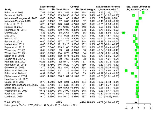
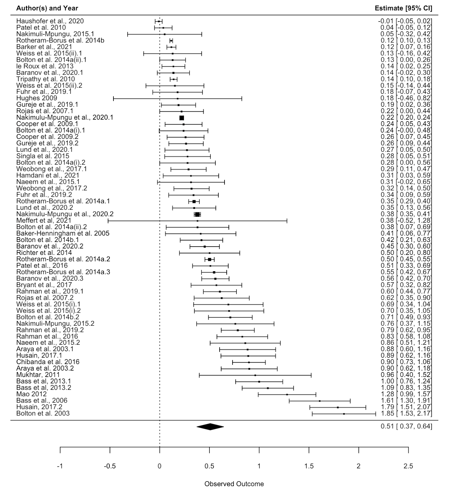
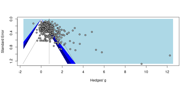
In the comments, Ryan Briggs and Gregory Lewis have pointed out that my meta-analysis of psychotherapy omits several typical and easy to produce figures. These are forest plots and funnel plots. A forest plot shows the individual study effects and the study effects. If I included this, it would have shown two things.
First, that there is quite a bit of variation in the effects between studies (i.e., heterogeneity). What heterogeneity implies is a bit controversial in meta-analyses, and I’ll return to this, but for now I’ll note that some take the presence of high heterogeneity as an indication that meta-analytic results are meaningless. At the other end of professional opinion, other experts think that high heterogeneity is often inevitable and merely warrants prudence. However, even the most permissive towards heterogeneity think that it makes an analysis more complicated.
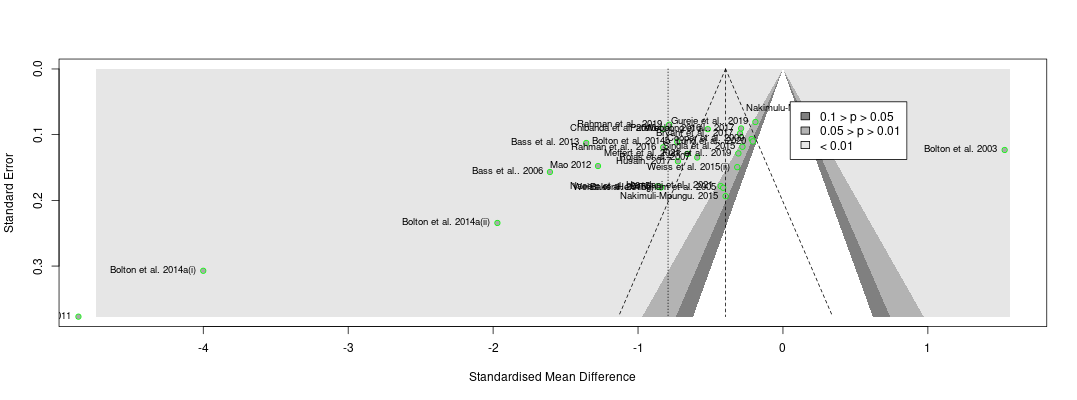
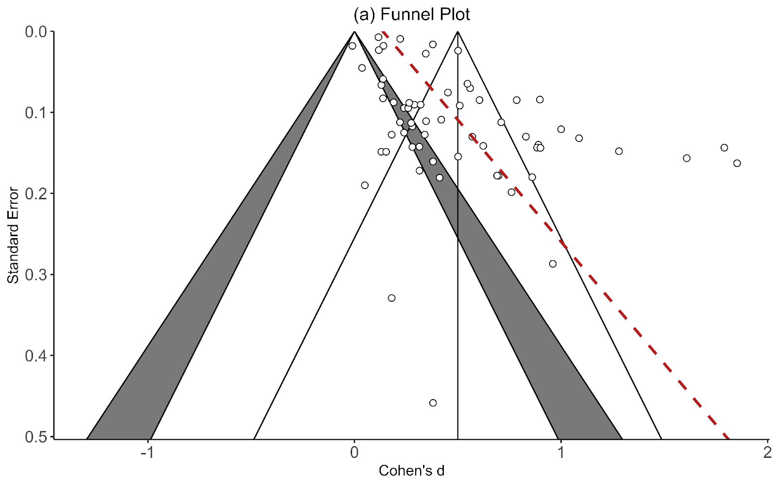
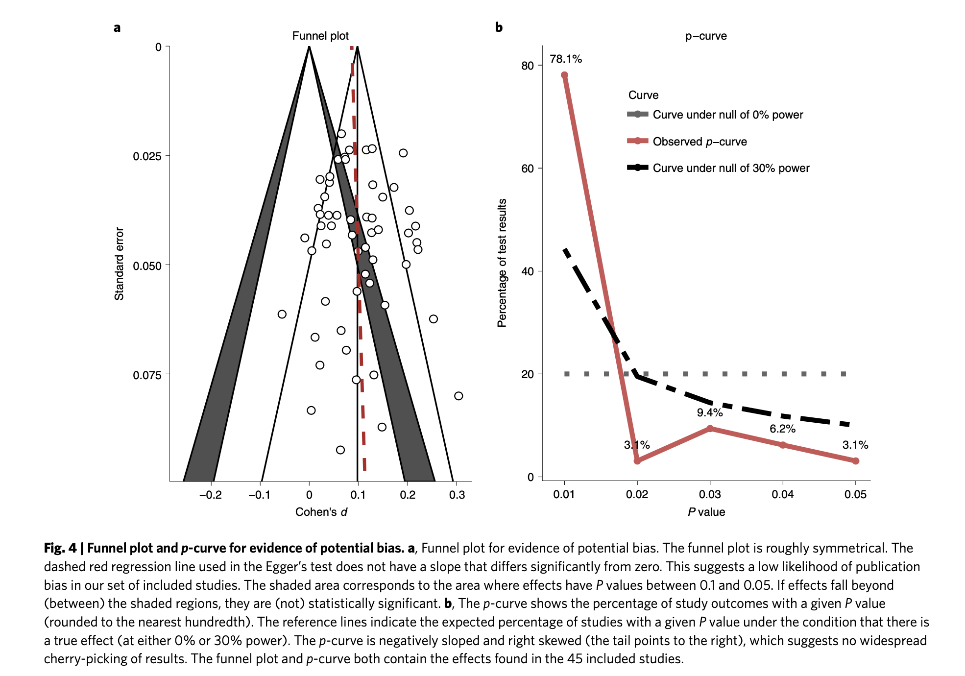
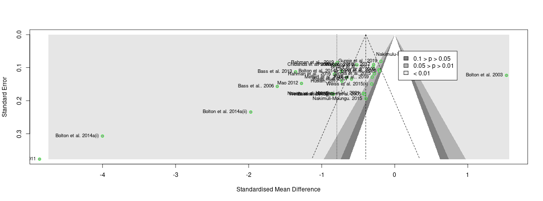
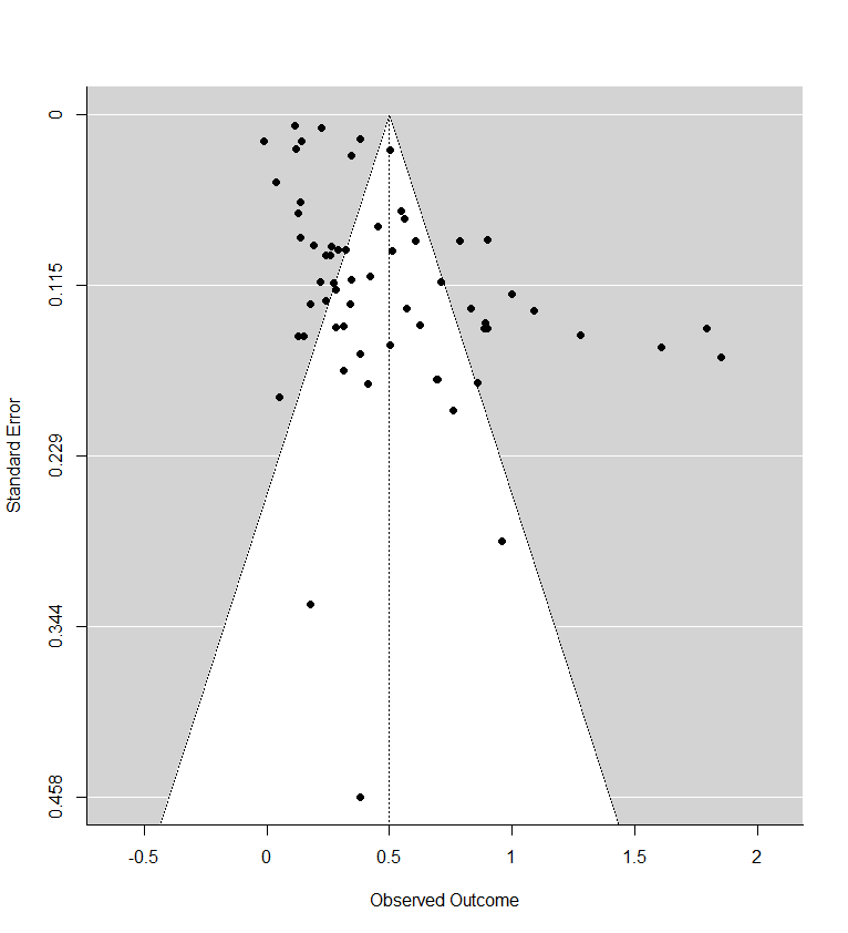
The second thing the forest plot shows is that there were a few considerable outliers. Notably, some of these outliers (Bolton et al., 2003; Bass et al., 2006) are part of the evidence I used to estimate that StrongMinds is more cost-effective than the typical psychotherapy intervention in LMICs. The other figure I omitted was a funnel plot. Funnel plots are made to show if there are many more small studies that find large effects than small with small, null or negative effects than we would expect due to a random draw. In the funnel plots for the psychotherapy data, which Gregory first provided by using a version of the the data I use, he rightly pointed out that there is considerable asymmetry, which suggests that there may be publication bias (i.e., the small sized studies that find small, null, or negative effects are less likely to be published and included than small studies with larger effects). This finding seemed all the more concerning given that I found pretty much no asymmetry in the cash transfers data I compare psychotherapy to.
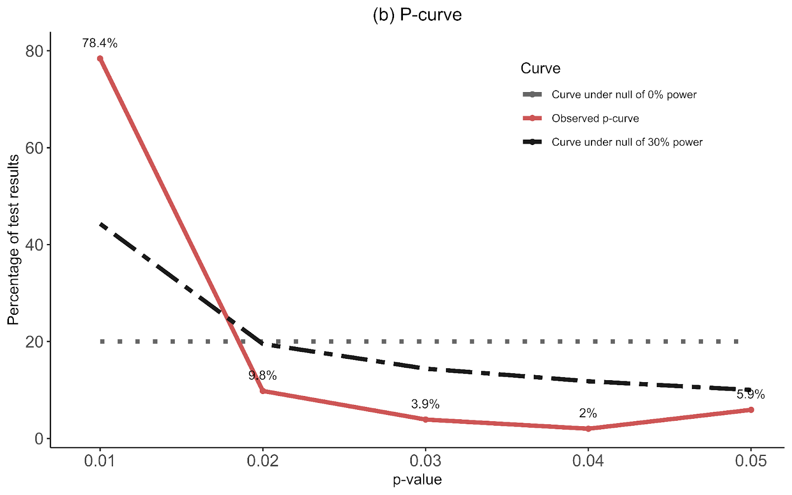
I supplemented this with a newer illustration, the p-curve, meant to detect publication bias that’s not just about the size of an effect, but its precision. The p-curve suggests publication bias if there’s an uptick in the number of effect sizes near the 0.05 significance level relative to the 0.03 or 0.04 level. The idea is that researchers are inclined to fiddle with their specifications until they are significant, but that they’re limited in their ambitions to perform questionable research practices and will tend to push them just over the line. The p-curve for psychotherapy shows a slight uptick near the 0.05 level, compared to none in cash transfers. This is another sign that the psychotherapy evidence base appears to have more publication bias than cash transfers.
Ryan and Gregory rightly pushed me on this – as I didn’t show these figures that make psychotherapy look bad. I have excuses, but they aren’t very good so I won’t repeat them here. I think it’s fair to say that these could have and should have been included.
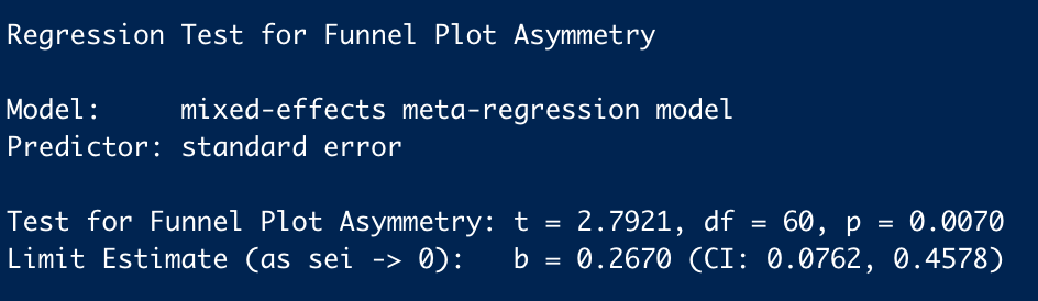
The next, and most concerning point that Ryan and Gregory made was that if we take the Egger regression test seriously (a formal, less eye-bally way of testing for funnel plot asymmetry), it’d indicate that psychotherapy’s effect size should be dramatically reduced[1]. This frankly alarmed me. If this was true, I potentially made a large mistake [2].
2. Does correcting for publication bias substantially change our results?
To investigate this I decided to look into the issue of correcting for publication bias in more depth. To do so I heavily relied upon Harrer et al. (2021), a textbook for doing meta-analyses in R.
My idea for investigating this issue would be to go through every method for correcting publication bias mentioned in Harrer et al. (2021) and show how these methods change the cash transfers to psychotherapy comparison. I thought this would be more reasonable than trying to figure out which one was the method to rule them all. This is also in line with the recommendations of the textbook “No publication bias method consistently outperforms all the others. It is therefore advisable to always apply several techniques…” For those interested in an explanation of the methods, I found Harrer et al. (2021) to be unusually accessible. I don’t expect I’ll do better.
One issue is that these standard approaches don’t seem readily applicable to the models we used. Our models are unusual in that they are 1. Meta-regressions, where we try to explain the variation in effect sizes using study characteristics like time since the intervention ended, and 2. Multi-level meta-analyses that attempt to control for the dependency introduced by adding multiple timepoints or outcomes from a single study. It doesn’t seem like you can easily plug these models into the standard publication bias methods. Because of this uncertainty we tried to run several different types of analyses (see details in 2.1) based on whether a model included the full data or excluded outliers or follow-ups or used a fixed or random effects estimator[3].
I ran (with the help of my colleague Samuel[4]) the corrections for both psychotherapy and cash transfers and then apply the percentage of correction to their cost-effectiveness comparison. It doesn’t seem principled to only run these corrections on psychotherapy. Even though the problem seems worse in psychotherapy, I think the appropriate thing to do is also run these corrections on the cash transfers evidence and see if the correction is greater for psychotherapy.
If you want to go straight to the raw results, I collected them in a spreadsheet that I hope is easy to understand. Finally, if you’re keen on replicating this analysis, we’ve posted the code we used here.
2.1 Model versions
Measures of heterogeneity and publication bias seem to be designed for simpler meta-analysis models than those we use in our analysis. We use a meta-regression with follow-up time (and sometimes dosage), so the estimate of the intercept is affected by the coefficients for time and other variables. Reading through Harrer et al. (2021) and a brief google search didn’t give us much insight as to whether these methods could easily apply to a meta-regression model. Furthermore, most techniques presented by Harrer et al. (2021) used a simple meta-analysis model which employed a different set of R functions (metagen rather than the rma.uni or rma.mv models we use).
Instead, we create a simple meta-analysis model to calculate the intercept for psychotherapy and for cash. We then apply the publication bias corrections to these models and get the % change this created. We then apply the % change of the correction to the effect for psychotherapy and cash and obtain their new cost-effectiveness ratio.
Hence, we are not using the model we directly use in our analysis, but we apply to our analysis the change in effectiveness that the correction method would produce on a model appropriate for said correction method.
Because of our uncertainty, we ran several different types of analyses based on whether a model included the full data[5] or excluded outliers[6] or follow-ups[7] or used a fixed or random effects estimator[8].
2.2 Results
The results of this investigation are shown below. Tests that are to the left of the vertical line represent decreases in the cost-effectiveness of psychotherapy relative to cash transfers. The reference models are the six right on the line (in turquoise). I’ll add further commentary below.
Details of the results can be seen in this spreadsheet. We removed tests 28, 29, 30, 34, 35, 36. These were generally favourable to psychotherapy. We removed them because they were p-curve and Rücker’s limit corrections models that we specified as fixed-effects models but they seemed to force the models into random-effects models, making their addition seem inappropriate[9].
Surprisingly, when we apply these tests, very few dramatically reduce the cost-effectiveness of psychotherapy compared to cash transfers, as indicated by changes to their intercepts / the estimated average overall effect.
2.3 Uncertainties
2.4 A note about heterogeneity
Sometimes it’s suggested that the high heterogeneity in a meta-analysis means it is impossible to interpret (see details of heterogeneity in my analyses in this spreadsheet). Whilst heterogeneity is important to report and discuss, we don’t think it disqualifies this analysis.
However, high levels of heterogeneity appear to be a common problem with meta-analyses. It’s unclear that this is uniquely a problem with our meta-analysis of psychotherapy. In their big meta-analysis of psychotherapy, Cuijpers et al. (2023; see Table 2) also have high levels of heterogeneity. Our cash transfer meta-analysis also has high (albeit lower than psychotherapy) levels of heterogeneity.
High heterogeneity would be very problematic if it meant the studies are so different they are not measuring the same thing. Alternative explanations are that (1) psychotherapy is a phenomenon with high variance (supported by similar findings of psychotherapy in HICs), and/or (2) studies about psychotherapy in LMICs are few and implemented in different ways, so we expect this data is going to be messy.
3. Next Steps
Note that the Egger regression is a diagnostic test, not a form of correction. However, the PET and PEESE methods are correction methods and are quite similar in structure to the Egger regression test.
Point taken that the omission is arguably, a non-trivial mistake.
Choosing a fixed or random effects model is another important and controversial question in modelling meta-analysis and we wanted to test whether the publication bias corrections were particularly sensitive to it. However, it seems like our data is not suitable to the assumptions of a fixed effects model – and this isn’t uncommon. As Harrer et al., (2021) say: “In many fields, including medicine and the social sciences, it is therefore conventional to always use a random-effects model, since some degree of between-study heterogeneity can virtually always be anticipated. A fixed-effect model may only be used when we could not detect any between-study heterogeneity (we will discuss how this is done in Chapter 5) and when we have very good reasons to assume that the true effect is fixed. This may be the case when, for example, only exact replications of a study are considered, or when we meta-analyze subsets of one big study. Needless to say, this is seldom the case, and applications of the fixed-effect model “in the wild'' are rather rare.”
If my analyses are better in the future, it's because of my colleague Samuel Dupret. Look at the increase in quality between the first cash transfer and psychotherapy reports and the household spillover report. That was months apart. You know what changed? Sam.
The same data we use in our full models.
Some methods are not robust to high levels of heterogeneity, which is more often present when there are outliers. We select outliers for the fixed and random effects models based on “‘non-overlapping confidence intervals’ approach, in which a study is defined as an outlier when the 95% confidence interval (CI) of the effect size does not overlap with the 95% CI of the pooled effect size” (Cuijpers et al., 2023; see Harrer et al., 2021 for a more detailed explanation).
We are concerned that these methods are not made with the assumption of a meta-regression and might react excessively to the follow-up data (i.e., effect sizes other than the earliest effect size collected in a study), which are generally smaller effects (because of decay) with smaller sample sizes (because of attrition).
Choosing a fixed or random effects model is another important and controversial question in modelling meta-analysis and we wanted to test whether the publication bias corrections were particularly sensitive to it. However, it seems like our data is not suitable to the assumptions of a fixed effects model – and this isn’t uncommon. As Harrer et al., (2021) say: “In many fields, including medicine and the social sciences, it is therefore conventional to always use a random-effects model, since some degree of between-study heterogeneity can virtually always be anticipated. A fixed-effect model may only be used when we could not detect any between-study heterogeneity (we will discuss how this is done in Chapter 5) and when we have very good reasons to assume that the true effect is fixed. This may be the case when, for example, only exact replications of a study are considered, or when we meta-analyze subsets of one big study. Needless to say, this is seldom the case, and applications of the fixed-effect model “in the wild'' are rather rare.”
The only tests that are different from the random effects ones are 32 and 38 because the list of outliers were different for fixed effects and random effects.
I expect to assign relatively lower weight to the StrongMinds specific evidence. I was leaning this direction since the summer, but these conversations -- particularly the push from Simon, hardened my views on this. This change would decrease the cost-effectiveness of StrongMinds. Ideally, I’d like to approach the aggregation of the StrongMinds specific and general evidence of lay-group psychotherapy in LMICs in a more formally Bayesian manner, but this would come with many technical difficulties. I will also look into the counterfactual impact of their scaling strategy where they instruct other groups in how to provide group psychotherapy.
Thanks for this, Joel. I look forward to reviewing the analysis more fully over the weekend, but I have three major concerns with what you have presented here.
1. A lot of these publication bias results look like nonsense to the naked eye.
Recall the two funnel plots for PT and CT (respectively):
I think we're all seeing the same important differences: the PT plot has markers of publication bias (asymmetry) and P hacking (clustering at the P<0.05 contour, also the p curve) visible to the naked eye; the CT studies do not really show this at all. So heuristically, we should expect statistical correction for small study effects to result in:
If a statistical correction does the opposite of these things, I think we should say its results are not just 'surprising' but 'unbelievable': it just cannot be true that, given the data we see being fed into the method it should lead us to conclude this CT literature is more prone to small-study effects than this PT one; nor (contra the regression slope in the first plot), the effect size for PT should be corrected upwards.
Yet many of the statistical corrections you have done tend to fail one or both of these basically-diagnostic tests of face validity. Across all the different corrections for PT, on average the result is a 30% increase in PT effect size (only trim and fill and selection methods give families of results where the PT effect size is reduced). Although (mostly) redundant, these are also the only methods which give a larger drop to PT than CT effect size.
As comments everywhere on this post have indicated, heterogeneity is tricky. If (generally) different methods all gave discounts, but they were relatively small (with the exception of one method like a Trim and Fill which gave a much steeper one), I think the conclusions you drew above would be reasonable. However, for these results, the ones that don't make qualitative sense should be discarded, and the the key upshot should be: "Although a lot of statistical corrections give bizarre results, the ones which do make sense also tend to show significant discounts to the PT effect size".
2. The comparisons made (and the order of operations to get to them) are misleading
What is interesting though, is although in % changes correction methods tend to give an increase to PT effect size, the effect sizes themselves tend to be lower: the average effect size across analyses is 0.36, ~30% lower than the pooled estimate of 0.5 in the funnel plot (in contrast, this is 0.09 - versus 0.1, for CT effect size).
This is the case because the % changes are being measured, not against the single reference value of 0.5 in the original model, but the equivalent model in terms of random/fixed, outliers/not, etc. but without any statistical correction technique. For example: row 13 (Model 10) is Trim-and-Fill correction for a fixed effect model using the full data. For PT, this effect size is 0.19. The % difference is calculated versus row 7 (Model 4), a fixed effect model without Trim-and-Fill (effect = 0.2) not the original random effects analysis (effect = 0.5). Thus the % of reference effect is 95% not 40%. In general, comparing effect sizes to row 4 (Model ID 1) generally gets more sensible findings, and also generally more adverse ones. re. PT pub bias correction:
In terms of (e.g.) assessing the impact of Trim and Fill in particular, it makes sense to compare like with like. Yet presumably what we care about to ballparking the estimate of publication bias in general - and for the comparisons made in the spreadsheet mislead. Fixed effect models (ditto outlier exclusion, but maybe not follow-ups) are already an (~improvised) means of correcting for small study effects, as they weigh them in the pooled estimate much less than random effects models. So noting Trim-and-Fill only gives a 5% additional correction in this case buries the lede: you already halved the effect by moving to a fixed effect model from a random effect model, and the most plausible explanation why fixed effect modelling limits distortion by small study effects.
This goes some way to explaining the odd findings for statistical correction above: similar to collider/collinearity issues in regression, you might get weird answers of the impact of statistical techniques when you are already partly 'controlling for' small study effects. The easiest example of this is combining outlier removal with trim and fill - the outlier removal is basically doing the 'trim' part already.
It also indicates an important point your summary misses. One of the key stories in this data is: "Generally speaking, when you start using techniques - alone or in combination - which reduce the impact of publication bias, you cut around 30% of the effect size on average for PT (versus 10%-ish for CT)".
3. Cost effectiveness calculation, again
'Cost effectiveness versus CT' is a unhelpful measure to use when presenting these results: we would first like to get a handle on the size of the small study effect in the overall literature, and then see what ramifications it has for the assessment and recommendations of strongminds in particular. Another issue is these results doesn't really join up with the earlier cost effectiveness assessment in ways which complicate interpretation. Two examples:
More important than this, though, is the 'percentage of what?' issue crops up again: the spreadsheet uses relative percentage change to get a relative discount vs. CT, but it uses the wrong comparator to calculate the percentages.
Lets look at row 13 again, where we are conducting a fixed effects analysis with trim-and-fill correction. Now we want to compare PT and CT: does PT get discounted more than CT? As mentioned before, for PT, the original random effects model gives an effect size of 0.5, and with T'n'F+Fixed effects the effect size is 0.19. For CT, the original effect size is 0.1, and with T'n'F +FE, it is still 0.1. In relative terms, as PT only has 40% of the previous effect size (and CT 100% of the effect size), this would amount to 40% of the previous 'multiple' (i.e. 3.6x).
Instead of comparing them to the original estimate (row 4), it calculates the percentages versus a fixed effect but not T'n'F analysis for PT (row 7). Although CT here is also 0.1, PT in this row has an effect size of 0.2, so the PT percentage is (0.19/0.2) 95% versus (0.1/0.1) 100%, and so the calculated multiple of CT is not 3.6 but 9.0.
The spreadsheet is using the wrong comparison, as we care about whether the multiple between PT and CT is sensitive to different analyses, relative sensitivity to one variation (T'n'F) conditioned on another (fixed effect modelling). Especially when we're interested in small study effects and the conditioned on effect likely already reduces those.
If one recalculates the bottom line multiples using the first model as the comparator, the results are a bit less weird, but also more adverse to PT. Note the effect is particularly reliable for T'n'F (ID 7-12) and selection measures (ID 37-42), which as already mentioned are the analysis methods which give qualitatively believable findings.
Of interest, the spreadsheet only makes this comparator error for PT: for CT, whether all or lumped (column I and L) makes all of its percentage comparisons versus the original model (ID 1). I hope (and mostly expect) this is a click-and-drag spreadsheet error (or perhaps one of my understanding), rather than my unwittingly recovering an earlier version of this analysis.
Summing up
I may say more next week, but my impressions are
I will try and summarise and comment on what I think are some possible suggestions you raise, which happen to align with your three sections.
1. Discard the results that don't result in a discount to psychotherapy [1].
If I do this, the average comparison of PT to CT goes from 9.4x --> 7x. That seems like a plausible correction, but I'm not sure it's the one I should use. I interpreted these results s as indicating none of the tests give reliable results. I'll quote myself:
I'm really unsure if 9.4x --> 7x is a plausible magnitude of correction. The truth of the perfect test could suggest a greater or smaller correction, I'm really uncertain given the behavior of these tests. That leaves me scratching my head at what principled choice to make.
I think if we discussed this beforehand and I said "Okay, you've made some good points, I'm going to run all the typical tests and publish their results." would you have said have advised me to not even try, and instead, make ad hoc adjustments. If so, I'd be surprised given that's the direction I've taken you to be arguing I should move away from.
2. Compare the change of all models to a single reference value of 0.5 [2].
When I do this, and again remove anything that doesn't produce a discount for psychotherapy, the average correction leads to a 6x cost-effectiveness ratio of PT to CT. This is a smaller shift than you seem to imply.
3. Fix the weighting between the general and StrongMinds specific evidence [3].
Gregory is referring to my past CEA of StrongMinds in guesstimate, where if you assign an effect size of 0 to the meta-analytic results it only brings StrongMinds cost-effectiveness to 7x GiveDirectly. While such behavior is permissible in the model, obviously if I thought the effect of psychotherapy in general was zero or close to, I would throw my StrongMinds CEA in the bin.
As I noted in my previous comment discussing the next version of my analysis, I said: " I expect to assign relatively lower weight to the StrongMinds specific evidence." To elaborate, I expect the effect estimate of StrongMinds to be based much more heavily on the meta-analytic results. This is something I already said I'd change.
I'll also investigate different ways of combining the charity specific and general evidence. E.g., a model that pins the estimates StrongMinds effects as relative to the general evidence. Say if the effects of StrongMinds are always say 5% higher, then if we reduce the effects of psychotherapy by from 0.5 to 0.1 then the estimate of StrongMinds would go from 0.525 to 0.105.
So what happens if we assign 100% of the weight to the meta-analytic results? The results would shrink by 20% [4]. If we apply this to the cost-effectiveness ratio that I so far think Gregory would endorse as the most correct (6x), this would imply a ~ 5x figure.
Is a reduction of 9.4x to 5x enough to make HLI pause its recommendation? As I said before:
Gregory rightly pointed out that we haven't made it clear what sort of reduction would result in us abandoning our recommendation of StrongMinds. I can't speak for the team, but for me this would definitely be if it was less than 1x GiveDirectly. The reason why this is so low is I expect our recommendations to come in grades, and not just a binary. My complete guess is that if StrongMinds went below 7x GiveDirectly we'd qualitatively soften our recommendation of StrongMinds and maybe recommend bednets to more donors. If it was below 4x we'd probably also recommend GiveDirectly. If it was below 1x we'd drop StrongMinds. This would change if / when we find something much more (idk: 1.5-2x?) cost-effective and better evidenced than StrongMinds.
However, I suspect this is beating around the bush -- as I think the point Gregory is alluding to is "look at how much their effects appear to wilt with the slightest scrutiny. Imagine what I'd find with just a few more hours."
If that's the case, I understand why -- but that's not enough for me to reshuffle our research agenda. I need to think there's a big, clear issue now to ask the team to change our plans for the year. Again, I'll be doing a full re-analysis in a few months.
4. Use a fixed effects model instead?
I'm treating this as a separate point because I'm not sure if this is what Gregory suggests. While it's true that fixed effects models are less sensitive to small studies with large effects, fixed effects models are almost never used. I'll quote Harrer et al., (2021) again (emphasis theirs):
I'm not an expert here, but I'm hesitant to use a fixed effects model for these reasons.
"However, for these results, the ones that don't make qualitative sense should be discarded, and the the key upshot should be: "Although a lot of statistical corrections give bizarre results, the ones which do make sense also tend to show significant discounts to the PT effect size".
"This is the case because the % changes are being measured, not against the single reference value of 0.5 in the original model, but the equivalent model in terms of random/fixed, outliers/not, etc. but without any statistical correction technique."
"On the guestimate, setting the meta-regressions to zero effect still results in ~7x multiples for Strongminds versus cash transfers."
We estimate the raw total effects of general psychotherapy to be 1.56 (see table 1) and 1.92 for StrongMinds (see end of section 4, page 18). 1.56/ 1.92 = 0.8125. The adjusted effects are smaller but produce a very similar ratio (1.4 & 1.7, table 2).
I have now had a look at the analysis code. Once again, I find significant errors and - once again - correcting these errors is adverse to HLI's bottom line.
I noted before the results originally reported do not make much sense (e.g. they generally report increases in effect size when 'controlling' for small study effects, despite it being visually obvious small studies tend to report larger effects on the funnel plot). When you use appropriate comparators (i.e. comparing everything to the original model as the baseline case), the cloud of statistics looks more reasonable: in general, they point towards discounts, not enhancements, to effect size: in general, the red lines are less than 1, whilst the blue ones are all over the place.
However, some findings still look bizarre even after doing this. E.g. Model 13 (PET) and model 19 (PEESE) not doing anything re. outliers, fixed effects, follow-ups etc, still report higher effects than the original analysis. These are both closely related to the eggers test noted before: why would it give a substantial discount, yet these a mild enhancement?
Happily, the code availability means I can have a look directly. All the basic data seems fine, as the various 'basic' plots and meta-analyses give the right results. Of interest, the Egger test is still pointing the right way - and even suggests a lower intercept effect size than last time (0.13 versus 0.26):
PET gives highly discordant findings:
You not only get a higher intercept (0.59 versus 0.5 in the basic random effects model), but the coefficient for standard error is negative: i.e. the regression line it draws slopes the opposite way to Eggers, so it predicts smaller studies give smaller, not greater, effects than larger ones. What's going on?
The moderator (i.e. ~independent variable) is 'corrected' SE. Unfortunately, this correction is incorrect (line 17 divides (n/2)^2 by itself, where the first bracket should be +, not *), so it 'corrects' a lot of studies to SE = 1 exactly:
When you use this in a funnel plot, you get this:
Thus these aberrant results (which happened be below the mean effect size) explain why the best fit line now points in the opposite direction. All the PET analyses are contaminated by this error, and (given PEESE squares these values) so are all the PEESE analyses. When debugged, PET shows an intercept lower than 0.5, and the coefficient for SE pointing in the right direction:
Here's the table of corrected estimates applied to models 13 - 24: as you can see, correction reduces the intercept in all models, often to substantial degrees (I only reported to 2 dp, but model 23 was marginally lower). Unlike the original analysis, here the regression slopes generally point in the right direction.
The same error appears to be in the CT analyses. I haven't done the same correction, but I would guess the bizarre readings (e.g. the outliers of 70x or 200x etc. when comparing PT to CT when using these models) would vanish once it is corrected.
So, when correcting the PET and PEESE results, and use the appropriate comparator (Model 1, I forgot to do this for models 2-6 last time), we now get this:
Now interpretation is much clearer. Rather than 'all over the place, but most of the models basically keep the estimate the same', it is instead 'across most reasonable ways to correct or reduce the impact of small study effects, you see substantial reductions in effect (the avg across the models is ~60% of the original - not a million miles away from my '50%?' eyeball guess.) Moreover, the results permit better qualitative explanation.
With that said, onto Joel's points.
1. Discarding (better - investigating) bizarre results
You are correct I would have wholly endorsed permuting all the reasonable adjustments and seeing what picture emerges. Indeed, I would be (and am) happy with 'throwing everything in' even if some combinations can't really work, or doesn't really make much sense (e.g. outlier rejection + trim and fill).
But I would have also have urged you to actually understand the results you are getting, and querying results which plainly do not make sense. That we're still seeing the pattern of "Initial results reported don't make sense, and I have to repeat a lot of the analysis myself to understand why (and, along the way, finding the real story is much more adverse than HLI presents)" is getting depressing.
The error itself for PET and PEESE is no big deal - "I pressed the wrong button once when coding and it messed up a lot of my downstream analysis" can happen to anyone. But these results plainly contradicted both the naked eye (they not only give weird PT findings but weird CT findings: by inspection the CT is basically a negative control for pub bias, yet PET-PEESE typically finds statistically significant discounts), the closely-related Egger's test (disagreeing with respect to sign), and the negative coefficients for the models (meaning they are sloping in the opposite direction) are printed in the analysis code.
I also find myself inclined to less sympathy here because I didn't meticulously inspect every line of analysis code looking for trouble (my file drawer is empty). I knew the results being reported for these analysis could not be right, so I zeroed in on it expecting there was an error. I was right.
2. Comparators
9.4x -> ~6x is a drop of about one third, I guess we could argue about what increment is large or small. But more concerning is the direction of travel: taking the 'CT (all)' comparator.
If we do not do my initial reflex and discard the PT favouring results, then we see adding the appropriate comparator and fixing the statistical error ~ halves the original multiple. If we continue excluding the "surely not" +ve adjustments, we're still seeing a 20% drop with the comparator, and a further 10% increment with the right results for PT PET/PEESE.
How many more increments are there? There's at least one more - the CT PET/PEESE results are wrong, and they're giving bizarre results in the spreadsheet. Although I would expect diminishing returns to further checking (i.e. if I did scour the other bits of the analysis, I expect the cumulative error is smaller or neutral), but the 'limit value' of what this analysis would show if there were no errors doesn't look great so far.
Maybe it would roughly settle towards the average of ~ 60%, so 9.4*0.6 = 5.6. Of course, this would still be fine by the lights of HLI's assessment.
3. Cost effectiveness analysis
Thank you for the benchmarks. However, I mean to beat both the bush and the area behind it.
The first things first, I have harped on about the CEA because it is is bizarre to be sanguine about significant corrections because 'the CEA still gives a good multiple' when the CEA itself gives bizarre outputs (as noted before). With these benchmarks, it seems this analysis, on its own terms, is already approaching action relevance: unless you want to stand behind cycling comparators (which the spreadsheet only does for PT and not CT, as I noted last time), then this + the correction gets you below 7x. Further, if you want to take SM effects as relative to the meta-analytic results (rather take their massively outlying values), you get towards 4x (e.g. drop the effect size of both meta-analyses by 40%, then put the SM effect sizes at the upper 95% CI). So there's already a clear motive to investigate urgently in terms of what you already trying to do.
The other reason is the general point of "Well, this important input wilts when you look at it closely - maybe this behaviour generalises". Sadly, we don't really need to 'imagine' what I would find with a few more hours: I just did (and on work presumably prepared expecting I would scrutinise it), and I think the results speak for themselves.
The other parts of the CEA are non-linear in numerous ways, so it is plausible that drops of 50% in intercept value lead to greater than 50% drops in the MRA integrated effect sizes if correctly ramified across the analysis. More importantly, the thicket of the guestimate gives a lot of forking paths available - given it seems HLI clearly has had a finger on the scale, you may not need many more relatively gentle (i.e. 10%-50%) pushes upwards to get very inflated 'bottom line multipliers'.
4. Use a fixed effects model instead?
As Ryan notes, fixed effects are unconventional in general, but reasonable in particular when confronted with considerable small study effects. I think - even if one had seen publication bias prior to embarking on the analysis - sticking with random effects would have been reasonable.
Gregory,
Thank you for pointing out two errors.
______________________________________________________
After correcting these errors, the picture does shift a bit, but the quantitative changes are relatively small.
Here's the results where only the change due to the publication bias adjusts the cost-effectiveness comparison. More of the tests indicate a downwards correction, and the average / median test now indicates an adjustment from 9.4x to 8x. However, when we remove all adjustments that favor PT in the comparison (models 19, 25, 23, 21, 17, 27, 15) the (average / median) is ratio of PT to CT is now (7x / 8x). This is the same as it was before the corrections.
Note: I added vertical reference lines to mark the 3x, 7x and 9.44x multiples.
Next, I present the changes where we include the model choices as publication bias adjustments (e.g., any reduction in effect size that comes from using a fixed effect model or outlier removal is counted against PT -- Gregory and Ryan support this approach. I'm still unsure, but it seems plausible and I'll read more about it). The mean / median adjustment leads to a 6x/7x comparison ratio. Excluding all PT favorable results leads to an average / median correction of 5.6x / 5.8x slightly below the 6x I previously reported.
Note: I added vertical reference lines to mark the 3x, 7x and 9.44x multiples.
Since the second approach bites into the cost-effectiveness comparison more and to a degree that's worth mentioning if true, I'll read more / raise this with my colleagues about whether using fixed effect models / discarding outliers are appropriate responses to suspicion of publication bias.
If it turns out this is a more appropriate approach, then I should eat my hat re:
The issue re comparators is less how good dropping outliers or fixed effects are as remedies to publication bias (or how appropriate either would be as an analytic choice here all things considered), but the similarity of these models to the original analysis.
We are not, after all, adjusting or correcting the original metaregression analysis directly, but rather indirectly inferring the likely impact of small study effects on the original analysis by reference to the impact it has in simpler models.
The original analysis, of course, did not exclude outliers, nor follow-ups, and used random effects, not fixed effects. So of Models 1-6, model 1 bears the closest similarity to the analysis being indirectly assessed, so seems the most appropriate baseline.
The point about outlier removal and fixed effects reducing the impact of small study effects is meant to illustrate cycling comparators introduces a bias in assessment instead of just adding noise. Of models 2-6, we would expect 2, 4,5 and 6 to be more resilient to small study effects than model 1, because they either remove outliers, use fixed effects, or both (Model 3 should be ~ a wash). The second figure provides some (further) evidence of this, as (e.g.) the random effects models (thatched) strongly tend to report greater effect sizes than the fixed effect ones, regardless of additional statistical method.
So noting the discount for a statistical small study effect correction is not so large versus comparators which are already less biased (due to analysis choices contrary to those made in the original analysis) misses the mark.
If the original analysis had (somehow) used fixed effects, these worries would (largely) not apply. Of course, if the original analysis had used fixed effects, the effect size would have been a lot smaller in the first place.
--
Perhaps also worth noting is - with a discounted effect size - the overall impact of the intervention now becomes very sensitive to linear versus exponential decay of effect, given the definite integral of the linear method scales with the square of the intercept, whilst for exponential decay the integral is ~linear with the intercept. Although these values line up fairly well with the original intercept value of ~ 0.5, they diverge at lower values. If (e.g.) the intercept is 0.3, over a 5 year period the exponential method (with correction) returns ~1 SD years (vs.1.56 originally), whilst the linear method gives ~0.4 SD years (vs. 1.59 originally).
(And, for what it is worth, if you plug in corrected SE or squared values in to the original multilevel meta-regressions, PET/PEESE style, you do drop the intercept by around these amounts either vs. follow-up alone or the later models which add other covariates.)
I will probably have longer comments later, but just on the fixed effects point, I feel it’s important to clarify that they are sometimes used in this kind of situation (when one fears publication bias or small study-type effects). For example, here is a slide deck from a paper presentation with three *highly* qualified co-authors. Slide 8 reads:
This is basically also my take away. In the presence of publication bias or these small-study type effects, random effects "are much more biased" while fixed effects are "also biased [...] but less so." Perhaps there are some disciplinary differences going on here, but what I'm saying is a reasonable position in political science, and Stanley and Doucouliagos are economists, and Ioannidis is in medicine, so using fixed effects in this context is not some weird fringe position.
--
(disclosure: I have a paper under review where Stanley and Doucouliagos are co-authors)
I may respond later after I’ve read more into this, but briefly — thank you! This is interesting and something I’m willing to change my mind about it. Also didn’t know about WAAP, but it sounds like a sensible alternative.