Executive summary: The post examines the long-run supply responsiveness of wild capture (fishing) versus aquaculture, highlighting that wild capture supply is typically less responsive to price and demand shifts compared to aquaculture due to factors like catch limits, fishing restrictions, and the natural limits of wild fish stocks.
Key points:
In the long run, firms can adjust various inputs like capital, labor, and production levels, but in the short run at least one input is often fixed.
Wild capture fisheries are often less responsive to price and demand shifts than aquaculture, with supply sometimes even changing in the opposite direction due to overfishing.
Fishery management policies like total allowable catch (TACs) can reduce the responsiveness of wild capture supply to price and demand shifts.
Estimates of own-price elasticities of supply tend to be lower for wild capture than aquaculture.
The effects of demand shifts on wild capture supply depend on the relative magnitudes of the supply and demand elasticities.
Supply elasticity estimates from the literature show wild capture elasticities are often lower and sometimes negative, while aquaculture elasticities tend to be higher and positive.
This comment was auto-generated by the EA Forum Team. Feel free to point out issues with this summary by replying to the comment, andcontact us if you have feedback.
The responsiveness of aquatic animal supply — EA Forum
This post is co-authored with Ben Garfinkel. It is cross-posted from the CEA blog. A PDF version can be found here.
Summary: Some strategic decisions available to the effective altruism m...
Disclaimer: Although I work on the Groups Team at CEA, I’m writing this in a personal capacity, and this post does not constitute an endorsement by CEA.
Agency - the realisation that you really can just do things.
TL;DR
Biosecurity needs people (of any background) who are agentic and have a high execution velocity and track record....
TL;DR: I'm releasing a website that ranks philanthropists according to EA principles and research, and allows users to re-rank the list using their own assumptions. I'd like feedback and help making it better. I'd especially like ideas for how to make the results more trustworthy. Funding may be available.
I recently built Impact List (impactlist.xyz), a site which ranks people by their positive impact via donations.
The goal is t...
Fishing is typically less responsive to price and demand shifts than aquaculture is, and in many wild fisheries, quite unresponsive overall on the margin. I discuss multiple reasons for this.
In some wild fisheries, lower prices and negative demand shifts for wild-caught species, e.g. from people going vegan or switching to plant-based substitutes, can actually cause their supply to increase. The price elasticity of wild capture supply in a fishery is negative when there’s overfishing and no management practices that limit the price-responsiveness of capture around those price levels.
Given that fished stocks seem more often overfished than underfished, this could suggest that attempts to reduce demand — negative demand shifts — will tend to increase catch on the margin.
I describe background on elasticities and illustrate a simple method to approximate the effects of price and demand shifts on production.
I list supply elasticity estimates from the literature for wild capture and aquaculture. There seem to be few estimates for wild capture.
Acknowledgements
Thanks to Brian Tomasik, Ren Ryba and Tori for their feedback on an earlier draft, and Saulius Šimčikas for his supervision on an earlier unpublished project. All errors are my own.
Fishery supply responsiveness
I take supply, market responses and elasticities to be in the ‘long run’, e.g. “long-run supply elasticity”, which is just long enough for no costs to be fixed, depends on the industry and I’d guess is typically less than a decade.[1] In the long run, firms (business, companies) can buy or sell capital (fishing vessels, barns, equipment), hire staff or let staff go, enter or exit the market, switch input factors, and otherwise change production levels.[2] If supply and demand were otherwise stable, then a permanent shift in either or prices leads supply and demand to gradually moving until it approximately reaches a new equilibrium, and the long run is long enough for this new equilibrium to be approximately reached. It’s long enough for the market to approximately stop reacting to the shift. For fishing, reaching economic equilibrium would also require the fishery to reach population and catch equilibrium. In practice, equilibrium may never actually be reached, but the long run measures the time it would take to move from one economic equilibrium to another in response to a permanent supply, demand or price shift.
In the ‘short run’, over a shorter period of time, they are not able to do all of these, and at least one of their input factors, often capital, is fixed.
The long run effects are more representative of the ongoing effects of lasting shifts in supply or demand.
Wild capture (wild catch, fishing) is typically less responsive to price and demand shifts than aquaculture is, and in many wild fisheries, quite unresponsive overall on the margin. There are several related reasons to expect this.
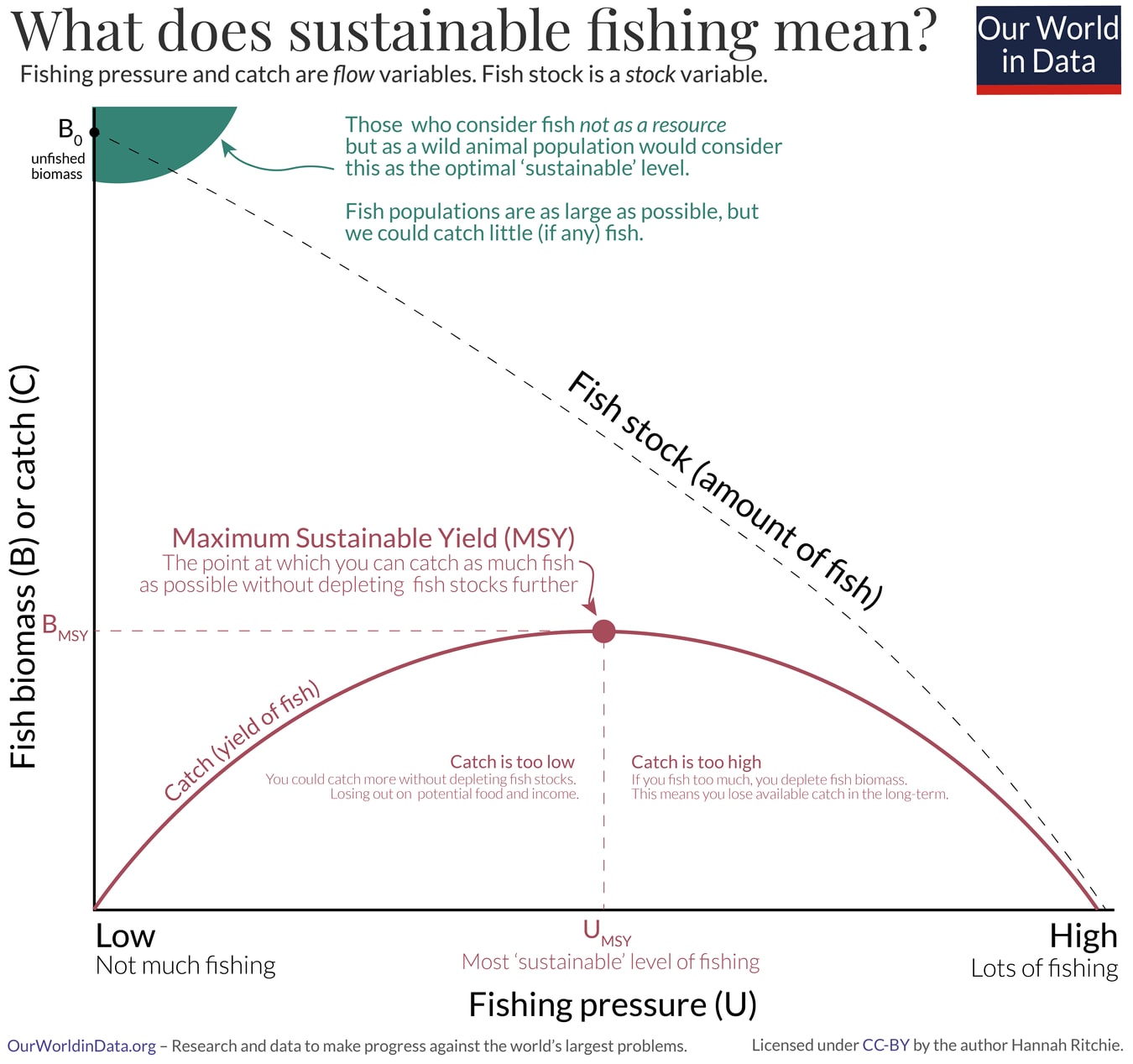
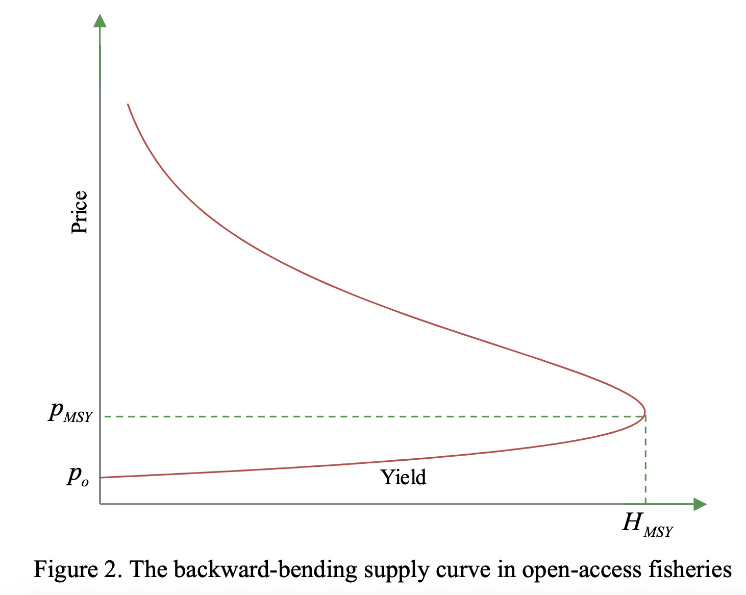
Credits: Ritchie & Roser, 2021–2024.Credits: Pham & Flaaten, 2013 (pdf). Unfortunately, economists like to graph price on the y axis and quantity produced on the x axis, instead of the more natural other way around.
H=harvest=C=catch, in weight per time period.
In open access (wild) fisheries — i.e. (wild) fisheries without policies restricting total catch and without responsive management, e.g. seasonal closures — supply increases as fishing pressure (or harvest rates)[3] or prices increase when they are less than those that achieve the maximum sustainable yield, barely responds near the maximum sustainable yield, and decreases when fishing pressure and prices are less than those that achieve the maximum sustainable yield, as illustrated in the two graphs above (Eide, 2012, Eide, 2011, Copes, 1970, Pham & Flaaten, 2013 (pdf), Ritchie & Roser, 2021–2024, Maximum sustainable yield - Wikipedia, Melnychuk et al., 2020, pp.9–16, Haddon, 2023, chapter 3). Inverse responsiveness, i.e. supply changing in the opposite direction as fishing pressure or prices, results from overfishing.
Wild aquatic animal stocks that are fished/exploited at all tend not to be underfished/underexploited, and are often approximately maximally sustainably fished or overfished/overexploited and have trended in this direction over time (FAO, 2022, Figure 23, Ritchie & Roser, 2021–2024). So, the responsiveness of catch to shifts in fishing pressure, prices or demand (see the next section) should usually be relatively small in magnitude or inverse in open access fisheries. However, this is by share of stocks, not weighed by the amount of catch, the number of individuals caught or the magnitudes of harms.
Several wild fishery management practices reduce the long-run responsiveness of capture supply to price and demand shifts compared to open access, typically to prevent or limit overfishing.
Governments set total allowable catch (TAC), the maximum allowed catch from a fishery or species in a fishery. These are often split into catch shares, granted across (or sold to, as quotas) fishers or fishing groups. We should expect the responsiveness to be close to 0 with properly enforced TACs when they are (approximately[4]) being met — when the TACs are binding.[5] TACs are implemented
for Peruvian anchoveta (Molinari, 2022, Molinari, 2024), who are the most wild-caught fish by volume and numbers, representing around 28% of the number of fish wild-caught annually on average (Mood & Brooke, 2024), and
increasingly, but with challenges, in China (Ding et al., 2023), the country that catches the most by tonnage, representing around 10% of global catch (Pauly et al./ Sea Around Us).
Governments may limit fishing vessel fleet sizes to specific targets to limit (but not entirely prevent, unless very low) overfishing across fisheries and species.
Governments may restrict fishing of given species in given fisheries in response to substantial stock or catch declines (due to overfishing), by reducing fleet sizes or seasonal closures, and loosen these restrictions upon stock recovery, e.g. closures for Peruvian anchoveta in 2023 (Evans, 2023, Molinari, 2023, Byrne, 2023) and 2020 (FAO, 2020).
Direct estimates of own-price elasticities of supply tend to be low for wild capture, and lower than for aquaculture, as in the last section.
Wild capture is effectively supply-limited by maximum sustainable yields (themselves limited by natural stocks and natural species population recovery). Aquaculture is limited more by feed availability and input prices, including feed prices, and while fishmeal is a major aquafeed ingredient, aquaculture continues to grow despite its limited supply, with shifts in aquaculture towards lower fishmeal inclusion rates in major fishmeal-consuming species (e.g. fishmeal inclusion rates have dropped from over 60% in 1990 to under 15% today, according to Barrows et al., 2023, Figure 1) and shifts towards herbivorous farmed species like carps and tilapias (FAO, 2022, p.43, Table 10, Hua et al., 2019 (alternative link), Figure 2).
Wild capture supply elasticities can be negative in some fisheries and positive in others, and negative and positive responses can partially cancel out when supply is aggregated across fisheries. This cancellation can bring the elasticity of aggregate wild capture supply closer to 0.
Note, however, that the effects of uniformly increasing or decreasing fishing pressure on the population sizes of species directly caught do not cancel out across fisheries, so an aggregate supply elasticity closer to 0 could hide large population effects.
Total annual wild capture has been relatively stable since the 1990s, while aquaculture production continues to grow and has overtaken capture (FAO, 2022, Figure 3). Annual capture for fishmeal has trended downwards since the 1990s, but with large fluctuations (Pauly et al./ Sea Around Us). In fact, World Bank, 2013 / Kobayashi et al., 2015 effectively set price elasticities of capture supply to 0 in part for this reason.[6]
Note that the local population effects of fishing — the effect on the number alive at any time — for the fished species tend to be much larger than the effects on their local annual catch, and fished species populations decrease with increasing fishing pressure, prices and demand in open access fisheries. And there are population effects for other species in the ecosystems to consider, too, e.g. prey, predators, competitors or parasites of the fished species, and others connected in the food web, which can go in either direction (Tomasik, 2015, Hulot et al., 2014, Eger & Baum, 2020, Christensen et al., 2014).
Elasticities and the impacts of demand shifts
The price elasticity of supply of a product, or own-price elasticity of supply of a product, or just supply elasticity of a product, is the the percentage change in the quantity supplied of the product caused by a small external (or “exogenous”) percentage shift (or “shock”) in the price of the product, divided by the percentage shift in the price, ϵ:
ϵ=%ΔQ%Δp,
where
%ΔQ=Q1−Q0Q0 is the percentage change in quantity supplied
%Δp=p1−p0p0 is the percentage shift in price
For example, if in response to a 2% positive shift in beef prices, beef production increased 1% annually in the long run, then the long-run price elasticity of beef supply would be around 0.5 = 1%/2%. If the short-run price elasticity of chicken meat were 0.7, then a -10% shift in chicken meat prices would cause a -7%=0.7*(-10%) reduction in chicken supply.
Supply elasticity estimates and demand elasticity estimates (defined similarly, but for demand instead of supply) can also be used to estimate the effects of an external shift in demand, e.g. people going vegan or otherwise reducing their consumption of the product for reasons other than changes to its price. In a simplified economic model of a competitive market with only a single product, we could estimate the expected effects of a small demand shift — small as a proportion of total quantity — on the quantity produced by multiplying the size of the demand shift by the factor
For example, if you get 1000 people to eliminate their combined consumption of X=10,000kg per year of wild-caught seafood from their diets, ϵS=0.1 and ϵD=−1 in the long run, then, in the long run, we’d expect supply of wild-caught seafood to drop by approximately
Because ϵD is typically negative, i.e. people want less of a product the more expensive it is, this multiplying factor increases with ϵS, except through ϵS=ϵD, where there is an asymptote (see this WolframAlpha graph). So, the more positive the supply elasticity, the larger the effect of the demand shift on actual production at equilibrium, all else equal.
If the supply elasticity is positive, i.e. ϵS>0, as is usually the case in most industries (fishing is often an exception), the factor E is positive and the quantity produced moves in the same direction as the demand shift.
If the supply elasticity is near 0, i.e. ϵS≈0, the factor E is also approximately 0, and there’s almost no effect from the demand shift, and none when the supply elasticity is exactly 0.
If the supply elasticity is negative (i.e. ϵS<0) and ϵS−ϵD>0, the factor E is negative and the actual effect of the demand shift on the quantity produced would be in the opposite direction of the demand shift, e.g. people going vegan causes more of the animal products to be produced.
If ϵS≈ϵD, the model breaks down, the factor E becomes very large in absolute value, and gives crazy answers, like the quantity produced increasing or decreasing many times more than the size of the shift, arbitrarily more the closer to equality and infinitely more at exact equality.
If ϵS−ϵD<0 (and ϵS<0), the factor E is positive, and the quantity produced moves in the same direction as the demand shift.
Substitution
In practice, however, we should also consider demand substitution effects between wild-caught aquatic animals and farmed animals. The effects of demand shifts for wild-caught aquatic animals could be larger on farmed animals than they are on wild-caught aquatic animals, at least by tonnes produced.
If two products are perfect substitutes in a competitive market, we can treat them as the same product with a common price after a unit conversion, add their supply curves together, and add their demand curves together. If one unit of product Y is equivalent to c units of product X, then measuring in equivalent units of product X, we could write the total supply of X and Y as
S(p)=SX(p)+cSY(p/c),
where SX(p) is the supply curve for X, the number of units of X produced if the price per unit of X is p, and SY(pY) is the supply curve for Y.
The price elasticity of the aggregate supply curve is the weighted average of the corresponding supply elasticities,
ϵS,X(p)SX(p)S(p)+ϵS,Y(p/c)SY(p/c)S(p)
where ϵS,X and ϵS,Y are the respective supply elasticities.[7] A weighted average works generally for more than 2 perfect substitutes for one another.
Then, we can estimate the effects of demand and price shifts on aggregate supply of X and Y as above, measured in equivalent units of X. We can estimate the effects on X and Y separately by estimating the percentage shift in equilibrium price, %Δp, e.g. as K/S(p)ϵS−ϵD with an external demand shift of absolute magnitude K so percentage shift of K/S(p) (Thomsen, 2018, Equation 4.3.1), and multiplying by the respective elasticities, giving relative shifts in equilibrium quantities of ϵX(p)∗%Δp and ϵY(p/c)∗%Δp.
I list estimates of price elasticity of supply of aquatic animal products I was able to find in the literature, where capture means wild capture (wild catch). I aimed to be pretty exhaustive in my search for wild capture elasticity estimates, but not for aquaculture.
Various estimates for China, South Asia and Southeast Asia in Dey et al., 2008:
0.2 to 0.48 for country averages in Table 8.2 Supply - Capture.
0.27 to 1.33 for country averages in Table 8.2 Supply - Aquaculture.
See also Table 7.15 for breakdowns by species groups, countries and capture vs aquaculture, which tend to be lower for capture than aquaculture. See also estimates in the appendices The World Fish Center, 2005.
Various long-run supply curves for anchovy capture in Vietnam in Pham & Flaaten, 2013 (pdf, Figure 4), for which supply elasticities at the prices used were negative (the backwards-bending parts of the supply curves).
According to Williams & Capps, 2020, for capture, "Studies using data before Norwegian fishery quota systems were fully binding found that the price elasticity of Norwegian fish supplies ranged from inelastic (Salvanes & Squires, 1995) to unitary elastic (Asche, 2009)."
Various (likely mistaken) estimates for capture in the long run: -9 to 4 for sea scallop, -30 to 500 for wreckfish, -0.08 to 0.065 for cod, -12 to 15 for surf clam and -50 to 20 for ocean quahog from figures 2 to 6 in Rudders & Ward, 2015. The estimates <-3 and >3 seem abnormally large and suspicious. I suspect they’re errors (e.g. due to biased estimation, possibly attributing natural variability to fishing, their unspecified “synthetic demand analysis”). Other possibilities could be that I’ve misinterpreted, or that the numbers are right and just reflect very high substitution between fishery products.
ExcludingRudders & Ward, 2015, aquaculture supply elasticities tend to be higher (more positive) than wild capture supply elasticities. And, of course, wild capture supply elasticity estimates are sometimes negative, but aquaculture supply elasticities are generally positive.
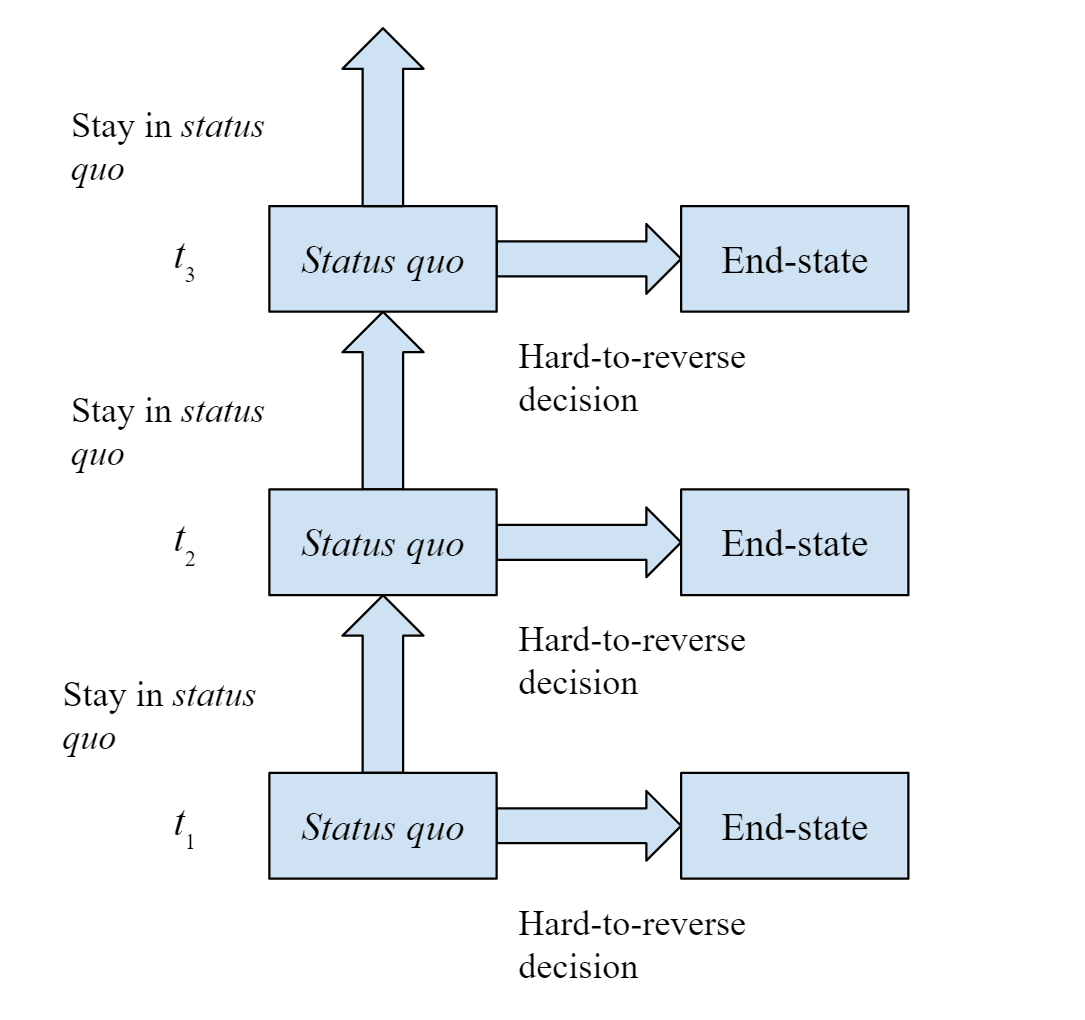
And it can depend on whether the production is increasing or decreasing. It seems faster to decrease production, e.g. shutting down businesses or factories, selling equipment, laying people off than to increase it, which may require capital construction or hiring, which take time. On the other hand, I could also imagine status quo bias, fear or attachment preventing industries from scaling down.
Furthermore, the long run is at least as long as the time to produce a new unit of product, which for animal agriculture, is at least the time between breeding an animal and the resulting offspring becoming productive, e.g. being slaughtered for food or feed, producing eggs or producing milk, because in response to an increase in price or demand for their products, there is a delay of at least this long before they can increase production to accommodate the new price level and demand.
Fishing pressure, also called the harvest rate, is the ratio, C/B, of catch, C, over the fishing period, in mass, to the biomass at the start of the fishing period, B.
Or, it's the ratio, C/N, of catch, C, over the fishing period, in number of individuals, to the population at the start of the fishing period, N. Some models use biomass and others use number of individuals.
This is not identical to the share of the biomass caught per period, and can actually be >1, because more animals will be born over the fishing period, the denominator is the biomass at the start of the period, and we can take fishing periods to be arbitrarily long.
Some allocated quotas may not be used for whatever reason. It’s unclear how price-responsive the share of allocated but unused is. Some may be unused due to poor planning on the part of the owner, or unforeseen circumstances, e.g. equipment breaking down.
If the supply function would be S(p) without a TAC, T is the TAC, and q(p,x) is the cost to fishers of the quota per unit of catch (if any, 0 otherwise), then with a TAC, the supply function would be
min(S(p−q(p,x)),T)
This function is constant when S(p−q(p,x))>T. If the TAC is met, i.e. min(S(p−q(p,x)),T)=T, it’s likely that S(p−q(p,x))>T, because S(p−q(p,x))=T exactly is very unlikely. So, catch is unlikely to be responsive to small price shifts when the TAC is met.
As seen in the previous section, the Fish to 2020 study tended to project overly optimistic growth of capture fisheries and underestimate the growth of aquaculture in relation to the actual data between 1997 and 2007. We suspect that the rising fish prices in the model, combined with capture supply that was specified overly sensitive to fish prices, drove the results. Consequently, the projected capture supply increased more than the actual data indicated, crowding out the growth of aquaculture in the model.
In response to these shortcomings, this study treats the growth of capture fisheries as entirely exogenous—that is, no supply response to price changes is modeled for capture fisheries. In terms of modeling price responses of supply, we maintain a solid focus on aquaculture. The rationale behind this decision is that, given relatively stable capture fisheries in the last decades and the fact that dynamic biological processes determine the amount of fish stock available for harvest, modeling of price-responsive capture supply in a static sense seems unrealistic. The open-access nature of many capture fisheries also further complicates the representation of fish supply behavior (Arnason, Kelleher, and Willmann 2009). Thus, rather than allowing capture supply to respond freely to increasing or decreasing fish prices, in this study we exogenously specify the behavior of capture fisheries based on the observed trends and according to alternative scenarios. However, results on the final distribution of capture fisheries production will depend on relative prices and demand in each country.
At equilibrium under the standard discrete Schaefer model (Haddon, 2023), the number caught per period is equal to the number of new individuals (recruitment) per period, after accounting for natural (or non-fishing) mortality,
C=rN(1−N/K),
Where
- C is the number of individuals caught per period,
- N is the number of individuals alive before capture in the period,
- U=C/N is the fishing pressure or harvest rate,
- K (or N0) is the carrying capacity of the stock in numbers of individuals, i.e. the natural/unfished population size, and
- r is the intrinsic rate (per period) of population increase, which reflects both fertility and natural mortality.
Then,
U∗N=C=rN(1−N/K)⇔U/r=1−N/K⇔N=K∗(1−U/r)
⇒dN/dU=−K/r
On the other hand,
C=U∗N=U∗K(1−U/r)=K(U−U2/r)
⇒dC/dU=K(1−2U/r)=K−2UK/r,
dC/dU reaches a maximum absolute value of K, at U=0 with value K and at U=r with value −K (U=r⇔N=0, and then dC/dU=−K). On the other hand, dC/dU is 0 at U/r=N/K=½, where equilibrium/sustainable catch is maximized as C=rK/4.
r is typically around 1 or smaller for a period of 1 year (e.g. Jensen et al., 2012 and Patrick & Cope, 2014) and |dC/dU|<K except with no fishing or an entirely eliminated stock, so typically K/r>K and |dN/dU|=K/r>K>|dC/dU|. I’d also expect |dC/dU| to be much less than K and so |dN/dU| in most fisheries, too, with C closer to its maximum sustainable (e.g. FAO, 2022, Figure 23, Ritchie & Roser, 2021–2024). However, there are disagreements over what model forms are best and hence and hence maximum sustainable yields.
Instead of numbers of individuals, biomass can be used, typically with notation B instead of N, and catch C and carrying capacity K would be measured in biomass (e.g. tonnes) rather than number of individuals, too.

Executive summary: The post examines the long-run supply responsiveness of wild capture (fishing) versus aquaculture, highlighting that wild capture supply is typically less responsive to price and demand shifts compared to aquaculture due to factors like catch limits, fishing restrictions, and the natural limits of wild fish stocks.
Key points:
This comment was auto-generated by the EA Forum Team. Feel free to point out issues with this summary by replying to the comment, and contact us if you have feedback.